|
"Curvature, Dummy Variables and Interaction" |
Index to Module Three Notes |
|
"Curvature, Dummy Variables and Interaction" |
Index to Module Three Notes |
Multiple regression gives us the capability to
add more than just numerical (also called quantitative) independent
variables. In these notes, we will examine the curvilinear
relationship between the dependent and independent variable, dummy
variables and interaction. To illustrate all three concepts, I want
to introduce a new example (I think I just heard some applause). Years Salary 13 72000 13 68000 10 66000 10 64000 14 64000 8 62000 15 61000 11 60000 9 60000 15 59000 5 59000 12 59000 11 58000 6 57000 7 56000 12 55000 6 55000 9 52000 14 51000 7 50000 3 45000 3 44000 4 44000 4 42000 8 41000 5 34000 2 34000 1 30000 2 25000 1 22000 SUMMARY OUTPUT Regression Statistics Multiple R 0.786315511 R Square 0.618292083 Adjusted R Square 0.604659658 Standard Error 8132.062603 Observations 30 ANOVA df SS MS F Significance F Regression 1 2999314286 2999314286 45.35451733 2.59764E-07 Residual 28 1851652381 66130442.18 Total 29 4850966667 Coefficients Standard Error t Stat P-value Lower 95% Upper 95% Intercept 33119.04762 3124.438012 10.6000015 2.61857E-11 26718.91929 39519.17594 Years 2314.285714 343.6423654 6.734576255 2.59764E-07 1610.365448 3018.20598
This example is near and dear to me: it involves a study of faculty
pay. Here is the data. Years of experience (Years) is the independent
variable hypothesized to predict Salary, the dependent variable.
Worksheet 3.2.1.
Review of Linear
Relationships
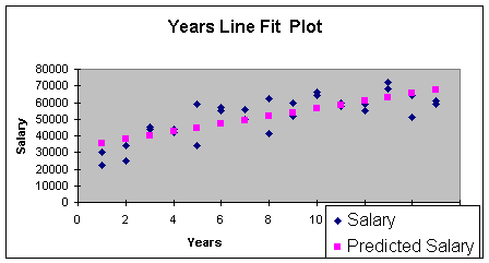
Suppose I wish to test a simple linear
relationship between Salary and Years. The scatter diagram with the
predicted linear regression equation is shown in the Worksheet 3.2.2
Line Fit Plot.
Worksheet 3.2.2
To determine if the linear regression has utility, I created the
regression summary shown in Worksheet 3.2.3 by using the Regression
Add-In Data Analysis Tool.
Worksheet 3.2.3
The Summary Output provides the linear regression equation intercept and slope:
Eq. 3.2.1: Salary = 33119 + 2314 (Years)
The intercept of $33,119 is the salary a
faculty member would make with no experience (a new hire). However, I
can't be sure of this since we did not have any years of experience
equal to zero in the sample. The slope of $2,314 indicates that
salary increases $2,314 for every year of experience.
Recall that our test for practical utility looks at R Square and the
Standard Error of the Model. The R Square is 0.62, meaning that Years
explain 62% of the sample variation in Salary in this linear model.
That is above the benchmark of 0.50. The correlation coefficient of
0.79 confirms the moderate strength. The standard error of $8,132
means that we would expect 95% of the actual salaries to be within
$16,264 (two times the standard error) of predicted salaries. This
seems a bit high for practical utility. We can hold that thought and
take a look at the assumptions.
To test for statistical utility, we set up the null and alternative
hypotheses:
H0: B1 = 0 (linear regression model is not statistically useful)
Ha: B1 =/= 0 (linear regression model is statistically useful)
Since the p-value (2.598E-07) for the t-Stat is
less than alpha of 0.05, we reject the null hypothesis and conclude
that the model has statistical utility.
To check the normality assumption for the errors or residuals, I
checked for outliers and there were none in the standardized residual
printout (I did not include these in Worksheet 3.2.2). Next, I
produced the residual plot to check for the assumptions of constant
error variance and independent errors. This is reproduced in
Worksheet 3.2.4.
Worksheet 3.2.4
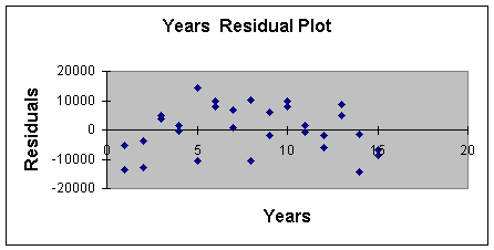
Note that for low values of Years, the
observations are below the zero error line, then mostly above the
line (up to 10), and then start to go back below the line of zero
error. This pattern indicates that the last two assumptions are not
satisfied and we may get a better model for prediction if we added
curvature.
Curvilinear
Relationships
The hypothesized regression model with
curvature is as follows:
Eq. 3.2.2: E(Y) = B0 + B1X + B2X2; for this example:Salary = B0 + B1(Years) + B2(Years)2
This equation is called the quadratic
equation. Years Years^2 Salary 13 169 72000 13 169 68000 10 100 66000 10 100 64000 14 196 64000 8 64 62000 15 225 61000 11 121 60000 9 81 60000 15 225 59000 5 25 59000 12 144 59000 11 121 58000 6 36 57000 7 49 56000 12 144 55000 6 36 55000 9 81 52000 14 196 51000 7 49 50000 3 9 45000 3 9 44000 4 16 44000 4 16 42000 8 64 41000 5 25 34000 2 4 34000 1 1 30000 2 4 25000 1 1 22000 SUMMARY OUTPUT Regression Statistics Multiple R 0.860591031 R Square 0.740616923 Adjusted R Square 0.721403361 Standard Error 6826.578401 Observations 30 ANOVA df SS MS F Significance F Regression 2 3592708005 1.8E+09 38.54657 1.22521E-08 Residual 27 1258258662 46602173 Total 29 4850966667 Coefficients Standard Error t Stat P-value Lower 95% Upper 95% Intercept 20961.53846 4299.678538 4.875141 4.26E-05 12139.33274 29783.74 Years 6605.171299 1236.600525 5.341395 1.22E-05 4067.878304 9142.464 Years^2 -268.1803491 75.15511808 -3.56836 0.00137 -422.3858105 -113.975
To add curvature, we simply create a new variable by squaring the
quantitative independent variable, as shown in Worksheet 3.2.5. On
the Excel Spreadsheet, I inserted a new column between Years and
Salary. Then in Cell B2, I entered the formula =A2*A2 (you could also
use the formula =A2^2) to get the squared term. I copied this down in
Column B to square all of the years.
Worksheet 3.2.5
Next, I got the Regression Summary by running the Regression Data
Analysis Add-In under the Tools icon on the Standard Toolbar,
just as we have done many times by now. Remember to increase your
selection for the X Range by including both columns of Years and
Years^2 (for Years Squared). The Regression Summary Results are shown
in Worksheet 3.2.6.
Worksheet 3.2.6
The coefficients for the multiple regression equation with curvature
are provided in the rows labeled Intercept, Years and Years^2. The
equation based on the sample is:
Eq. 3.2.3: Salary = 20961.5 + 6605.2 (Years) - 268.18 (Years)2
The intercept may be interpreted similar to simple linear
regression. Salary is $20,961.5 for faculty with no years of service
in this curvilinear model. Again, this is not a practical
interpretation since we had no faculty with zero years of service in
the data base.
The coefficient for Years Squared (-268.18) is a negative number
meaning that the curvature is negative. The interpretation of the
negative curvature is simply that as Years (X) increase, Salary (Y)
increases at a decreasing rate. Note that a positive
coefficient on the curvature variable would mean that as X increases,
Y increases at an increasing rate. The coefficient for Years,
6605.2, has no managerial interpretation. It simply locates the curve
on the XY axis.
Let's look at the line fit plot to see what negative curvature looks
like (Worksheet 3.2.7). As you recall, the line fit plot is part of
the automatic output of the Regression Add-In provided you check the
Line Fit Plot Residual Output Option.
Worksheet 3.2.7
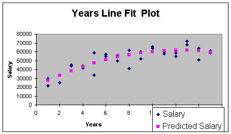
There is actually a name for the negative curve
shape - it's called concave. Positive curve shape looks like a
cross section of a bowl - it's called convex.
This model has better practical utility than the simple linear
regression model. The Adjusted R Square climbed to 0.72, compared to
0.62 for the simple linear regression model. The Standard Error
decreased from $8,132 to $$6,828. Still high, but it's an
improvement.
To test for statistical utility, we can first do a model
test.
H0: B1 = B2 = 0 (regression model is not statistically useful)
Ha: at lease one B =/= 0 (regression model is statistically useful)
Since the p-value (1.22521E-08) for the F is less than alpha of 0.01, we reject the null hypothesis and conclude that the model is statistically useful. Now, for our test on curvature. The hypotheses are:
H0: B2 = 0 (curvature is not important or curvature is not present)
Ha: B2 =/= 0 (curvature is important)
Since the p-value for the t-stat for the
Years^2 curvature term is less than alpha of 0.01, we reject the null
hypothesis and conclude that curvature is important. Since
Years^2 is important, we do not need to do a
separate test on Years since the Years variable is required to
produce Years^2.
To check the normality assumption for the errors or residuals, I
checked for outliers and there were none in the standardized residual
printout (I did not include these in Worksheet 3.2.6 ). Next, I
produced the residual plot to check for the assumptions of constant
error variance and independent errors. This is reproduced in
Worksheet 3.2.8.
Worksheet 3.2.8.
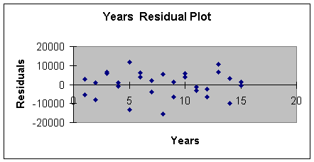
Although the magnitude of the variation starts small, gets larger,
gets small again and so forth, adding curvature did remove the
negative/positive/negative pattern. We will see even more improvement
when we add the categorical or dummy variable.
The last step in the regression procedure is to make the prediction.
Suppose we want to predict the salary for a professor with 10 years
experience. The point estimate is:
Eq. 3.2.4: Salary = 20961.5 +6605.2 (10) -268.18 (10)2 = $60,196
Adding the prediction interval gives us the following. We are 95% confident that a faculty member with 10 years experience will make a salary between $46,542 and $73,850, as shown in Eq. 3.2.5.
Eq. 3.2.5: Salary = $60,196 +/- (2 * Standard Error of Model)Salary = $60,196 +/- (2 * $6,827)
Salary = $60,196 +/- $13,654
Next we will examine categorical or dummy
variables.
Dummy Variables
Multiple regression gives us the
capability to incorporate a very useful technique to stratify the
data in our attempt to build more reliable and accurate prediction
models. We stratify data by using dummy variables (also called
categorical or qualitative variables).
Recall that the Standard Error of the Estimate of $6,827 for the
curvilinear model is fairly high, even though it is much better than
the Standard Error of the linear model. One reason that the error may
be so high is that I am including both male and female faculty member
in the database. If there is salary discrimination, combining both
males and females would lead to high error. One solution is to run
two separate models - one for females and one for males. Another
option is to stratify or categorize males and females in one
regression model. The benefit of stratification in one regression
model is that we picture any differences in the line fit plots, and
we can test for interaction which I cover last in this note set.
The way we stratify data is to categorize it by using a dummy
variable. In this case, let's let X represent a variable called
gender. It's values are:
X = 1 if the faculty member is male
X = 0 if the faculty member is female
Which gender gets the 1 and which gets the 0 is
arbitrary, but only use 1 and 0 for the two categories (for example,
do not use 2 and 1). Note that by using 0, the intercept will now
have an interpretation. Worksheet 3.2.9 illustrates the data for a
regression model with one dependent variable, Salary, and one
independent variable, gender. Gender Salary 1 72000 0 68000 1 66000 0 64000 1 64000 1 62000 1 61000 0 60000 1 60000 0 59000 1 59000 1 59000 1 58000 0 57000 1 56000 0 55000 1 55000 0 52000 0 51000 0 50000 1 45000 0 44000 1 44000 0 42000 0 41000 0 34000 1 34000 1 30000 0 25000 0 22000 SUMMARY OUTPUT Regression Statistics Multiple R 0.264756482 R Square 0.070095995 Adjusted R Square 0.036885137 Standard Error 12692.70507 Observations 30 ANOVA df SS MS F Significance F Regression 1 340033333.3 340033333.3 2.110634902 0.157394431 Residual 28 4510933333 161104761.9 Total 29 4850966667 Coefficients Standard Error t Stat P-value Lower 95% Upper 95% Intercept 48266.66667 3277.242356 14.72782951 1.03073E-14 41553.53248 54979.80085 Gender 6733.333333 4634.720587 1.45280243 0.157394431 -2760.472079 16227.13875
Worksheet 3.2.9
The first faculty member is a male making $72,000 (must be in the
College of Medicine or Engineering), the second faculty member is a
female, etc.
Worksheet 3.2.10 provides the regression Summary Output.
Worksheet 3.2.10
The regression Summary Output provides the following regression equation:
Eq. 3.2.6: E(y) = b0 + b1x ; for this sample:Salary = $48,267 + $6,733(Gender)
Recall that males were given the category 1 and females 0. So we can now make our point estimates of average male and female salaries:
Eq. 3.2.7: Salary = $48,267 + ($6,733 * 1) or $55,000 for males;Salary = $48,267 + ($6,733 * 0) or $48,267 for females
The regression parameters take on a different
interpretation for dummy variables. The "intercept" is the average
salary made by females, and the "slope" is the difference between the
average salaries made by males and females. Another difference with
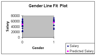
dummy variables is the line fit plot, since X only takes on values of
0 and 1. The line fit plot will show the cluster of female and male
faculty actual observations at X = 0 and X = 1, and the prediction
(average value for Y when X = 1, and average value for Y when X = 0)
as points. Worksheet 3.2.11 illustrates the line fit plot.
Worksheet 3.2.11
Generally, we use a dummy variable as a stratification variable along
with one or more other independent variables. Indeed, you can see
from the regression summary output that the regression model with
just gender and salary does not have statistical or practical
utility. We will combine the dummy variable with the experience
independent variable in the next section to see if our results
improve. I simply used the dummy variable by itself to introduce the
concept.
Dummy variables are used to categorize data in models where there are
attributes such as in season/out of season, large/small, and
defective/not defective. You will be asked to incorporate a dummy
variable in Assignment 3.
If the characteristic being modeled has more than two levels, we need
to use more than one dummy variable. For example, what if you wanted
to model Fall, Winter, Spring, Summer. Then, X1 could
represent Fall and if the observation is a Fall observation, it gets
the value 1 in data entry, 0 otherwise; X2 is used for
Winter; and X3 is used for Spring. There would be no dummy
variable for Summer. Do you know why? Did I hear, "the intercept
becomes Summer"? That's right!
For Assignment 3, we will be adding just one dummy variable, so keep
to two levels (male/female, in season/out of season, large/small,
etc.) .
The next modeling concept is interaction.
Interaction
When there are two independent
variables, the relationship between Y and X1 may depend on
X2: that dependency is called interaction. When the
relationship between Y and X1 does not depend on
X2 we say there is no interaction. I am going to
illustrate the "no interaction" case first, since I can use the data
in the faculty salary example. I will introduce a new data set to
demonstrate "interaction" after that.
The hypothesized population equation to model interaction
is:
Eq. 3.2.8: E(Y) = B0 + B1X1 + B2X2 + B3X1X2;
The cross-product term,
X1X2, is the interaction term, so B3
in Equation 3.2.8 is the slope of interest for testing
interaction. Years Gender Yrs*Gndr Salary 13 1 13 72000 13 0 0 68000 10 1 10 66000 10 0 0 64000 14 1 14 64000 8 1 8 62000 15 1 15 61000 11 0 0 60000 9 1 9 60000 15 0 0 59000 5 1 5 59000 12 1 12 59000 11 1 11 58000 6 0 0 57000 7 1 7 56000 12 0 0 55000 6 1 6 55000 9 0 0 52000 14 0 0 51000 7 0 0 50000 3 1 3 45000 3 0 0 44000 4 1 4 44000 4 0 0 42000 8 0 0 41000 5 0 0 34000 2 1 2 34000 1 1 1 30000 2 0 0 25000 1 0 0 22000 SUMMARY OUTPUT Regression Statistics Multiple R 0.830657322 R Square 0.689991587 Adjusted R Square 0.654221386 Standard Error 7605.262541 Observations 30 ANOVA df SS MS F Significance F Regression 3 3347126190 1115708730 19.28956392 8.62451E-07 Residual 26 1503840476 57840018.32 Total 29 4850966667 Coefficients Standard Error t Stat P-value Lower 95% Upper 95% Intercept 28809.52381 4132.381497 6.971651536 2.10919E-07 20315.28642 37303.76119 Years 2432.142857 454.5013685 5.351233298 1.33311E-05 1497.901302 3366.384412 Gender 8619.047619 5844.069958 1.474836489 0.152263821 -3393.618092 20631.71333 Yrs*Gndr -235.7142857 642.7619995 -0.366720942 0.716794859 -1556.931363 1085.502792
To model interaction with sample data, we multiple the two
independent variables to make a new variable. Worksheet 3.2.12
illustrates multiplying the contents of the cells in Column A (Years)
with the cells in Column B (Gender) to make a new variable,
Yrs*Gndr.
Worksheet 3.2.12
Worksheet 3.2.14 provides the regression Summary Output.
Worksheet 3.2.14
The coefficients for the multiple
regression model with interaction are provided in the rows labeled
Intercept, Years, Gender and Yrs*Gndr. The equation based on this
sample is:
Eq. 3.2.9: E(y) = b0 + b1x1 + b2x2 + b3x3 + b4x1x2; hereSalary = 28809.5 + 2432.1 (Years) +
8619 (Gender) - 235.7 (Yrs*Gndr)
To determine if interaction is important, we can proceed directly to the hypothesis test for interaction:
H0: B3 = 0 (interaction is not important)
Ha: B3 =/= 0 (interaction is important)
Since the p-value (0.717) for the t-stat for
the Yrs*Gndr term is greater than 0.01, we do not reject the null
hypothesis and conclude interaction is not important. The analyst
should then remove the interaction column of data and rerun the
regression model without interaction to see if either years or gender
or both are important in predicting salary. Worksheet 3.2.15
illustrates what "no interaction" looks like:
Worksheet 3.2.15
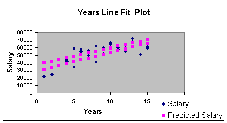
This line fit plot illustrates the relationship between Salary and
Years. But note that there are two regression lines. The two
regression lines represent the stratification of the data - one line
for males and one for females. Can you guess which is the top line?
Right - the male regression line is the top line. We learned that
when we examined the gender variable in the previous section: males
make more than females. There was, in fact, salary discrimination at
the university where this data sample came from.
But because the two regression lines have approximately the same
slope, we can predict the increase in salary for males or
females based on time alone. I realize that males make more than
females - but it is a fixed amount because the slopes are parallel.
Thus, the formal definition of "no interaction" is, for this problem:
the relationship between Salary and Years does not depend on
gender. Recall that statistical relationships between variables in
regression is measured through the slope. The slope on years is
$2,432 for both males and females since the Years*Gender term goes
away (the interaction slope is equal to zero).
IF there was interaction, then the slopes would be different
for males and females. For an hypothetical example, what if
the Equation 3.2.9 came out as follows:
Eq. 3.2.10: Salary = 28809.5 + 2432.1 (Years) + 8619 (Gender) +1000 (Yrs*Gndr)
Now note what happens when we substitute 1 (for males) in the gender term:
Eq. 3.2.11: Male Salary = 28809.5 + 2432.1 (Years) + 8619 (1) +1000 (1 * Years) = 37428.5 + 3432.1 (Years)...and then 0 (for females) in the gender term
Eq. 3.2.12: Female Salary = 28809.5 + 2432.1 (Years) + 8619 (0)+1000 (0 * Years) = 28809.5+ 2432.1 (Years)
In my hypothetical example, the slope for the
male regression line is 3432.1; meaning that male salaries increase
$3,432 per year. The slope for the female regression line is
$2,432.1; meaning that female salaries increase only $2,432.1 per
year. Since the slopes are different, we cannot predict the change in
salary without knowing the gender. Thus, we would say there is
interaction: the relationship between salary and years depends
on whether the faculty member is male or female. Age Drug Age*Drug Effect 21 1 21 56 19 0 0 28 28 1 28 55 23 0 0 25 67 0 0 71 33 1 33 63 33 1 33 52 56 0 0 62 45 0 0 50 38 1 38 58 37 0 0 46 27 0 0 34 43 1 43 65 47 0 0 59 48 1 48 64 53 1 53 61 29 0 0 36 53 1 53 69 58 1 58 73 63 1 63 62 59 0 0 71 51 0 0 62 67 1 67 70 63 0 0 71 SUMMARY OUTPUT Regression Statistics Multiple R 0.96551637 R Square 0.932221861 Adjusted R Square 0.92205514 Standard Error 3.87724774 Observations 24 ANOVA df SS MS F Significance F Regression 3 4135.297333 1378.432444 91.69346477 7.33335E-12 Residual 20 300.6610008 15.03305004 Total 23 4435.958333 Coefficients Standard Error t Stat P-value Lower 95% Upper 95% Intercept 6.211381194 3.308965648 1.877136802 0.075164685 -0.690996989 13.11375938 Age 1.033390871 0.071447502 14.46363902 4.70078E-12 0.884354064 1.182427679 Drug 41.30421013 5.022786373 8.223365889 7.5975E-08 30.82686622 51.78155404 Age*Drug -0.702883614 0.10763568 -6.530210205 2.30245E-06 -0.927407604 -0.478359625
The above illustration of interaction was hypothetical. There really
was no interaction but there really was discrimination - males made
more on average than females, but that amount was constant for all
levels of experience (no interaction). If the amount was not
constant, there would have been interaction).
Let's examine an actual model of interaction so you can an actual
picture and the equations for interaction. This example was an
experiment done by an over-the-counter drug manufacturer interested
in testing a new drug designed to be effective in curing an illness
most commonly found in older patients. The dependent variable is
Effect, which stands for the effectiveness of recovery from a certain
illness. It is measured on a scale of 0 to 100 (100 is more
effective). The quantitative independent variable is age, and the
qualitative independent variable is whether or not the new drug was
present (drug = 0) or absent (subjects took the old drug) (drug = 1)
in the experiment. Note that half of the subjects were given the new
drug, and half were given the old drug (they were not told which one
to avoid bias in the experiment. This would then be called a
blind experiment since the subjects did not know which drug
they were taking. An experiment is called a double blind
experiment if the drug administrator does not know which drug is
being administered, as well. Worksheet 3.2.16 shows the data
entry.
Worksheet 3.2.16
Worksheet 3.2.17 provides the regression summary.
Worksheet 3.2.17
The Intercept, Age, Drug and Age*Drug
regression coefficients provide the equation from this
sample:
Eq. 3.2.13: Effect = 6.2+ 1.03 (Age)+ 41.3 (Drug) - 0.7 (Age*Drug)
Let's look at the equation for subjects who got the old drug (did not get the new drug) (drug = 1):
Eq. 3.2.14: Effect = 6.2 + 1.03 (Age) + 41.3 (1) - 0.7 (Age*1)Effect = 47.5 + 0.33 (Age)
Now, look at the equation for subjects who got the new drug (drug = 0):
Eq. 3.2.15: Effect = 6.2 + 1.03 (Age) + 41.3 (0) - 0.7 (Age*0)Effect = 6.2 + 1.03 (Age)
Subjects who got the new drug would enjoy a
nearly a 1 unit increase in drug healing effectiveness for each year
of age. On the other hand, subjects who got the old drug only enjoy a
.33 unit increase in effectiveness for each year of age. The drug
manufacturer would be excited about this finding - the new drug is
more effective as one ages. Statistically, we say there is
interaction. The relationship between effectiveness and age depends
on whether or not the subject is taking the drug. The slopes of the
regression equation change when there is interaction.
Worksheet 3.2.18
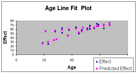
In the Worksheet 3.2.18 Line Fit Plot, note the steeper sloping line
that begins with the observation of a subject aged 20, with an
effectiveness score of just below 30. This is the line of Equation
3.2.15 - the one with the steeper slope that shows more effectiveness
with age than line of Equation 3.2.14. The drug manufacturer can then
tell that for subjects over 60, there should be more effectiveness in
healing with the new drug as patients age. I will use this example
again in Module Notes 3.2.3 when we discuss model building. I will go
over statistical and practical utility, testing assumptions and
prediction with this model at that time. This illustration was simply
used to show a picture of interaction.
That's it! We now talked about the separate components of multiple
regression. Adding a quantitative independent variable, adding a
qualitative (dummy) independent variables, adding a curvature
component, and adding an interaction component. There can be more
complications - such as adding several more quantitative variables
and studying three-way interactions - but you have the basic building
blocks of multiple regression involving a quantitative dependent
variable. Note that because of the principle of parsimony,
I would suggest caution before building a model that has so many
terms it is impossible to interpret.
There are model extensions for qualitative dependent variables but
they go beyond the scope of this course.
All that remains for our study of multiple regression is a system for
knowing how to put the separate components together in a single
model. That is the subject of Module Notes 3.3.
References:
Anderson, D., Sweeney, D., &
Williams, T. (2001). Contemporary Business Statistics with Microsoft
Excel. Cincinnati, OH: South-Western, Chapter 12 (Section
12.9).
Levine, D., Berenson, M. & Stephan,
D. (1999). Statistics for Managers Using Microsoft Excel (2nd.
ed.). Upper Saddle River, NJ: Prentice-Hall.
Chapter 14 -- Multiple Regression Models
Mason, R., Lind, D. & Marchal, W. (1999). Statistical
Techniques in Business and Economics (10th. ed.).
Boston: Irwin McGraw Hill.
Chapter 13 -- Multiple Regression and Correlation Analysis
|
|
|
|