"If you know a thing only qualitatively, you know it no more than vaguely…If you know it quantitatively--grasping some numerical measure that distinguishes it from an infinite number of other possibilities--you are beginning to know it deeply…You comprehend some of its beauty and you gain access to its power and the understanding it provides…"

Carl Sagan (1997), "Billions and Billions: Thoughts on Life and Death At the Brink of the Millennium."

Let's move this thought into a business world example to introduce statistics for managers. Don't worry about how to do the computations - we will cover that later. For now, just focus on the concepts illustrated in this introduction.

... If you don't know a process quantitatively, you run the risk of making at least two errors (D. Wheeler, 1993).

The first error is to interpret noise as if it were a signal.

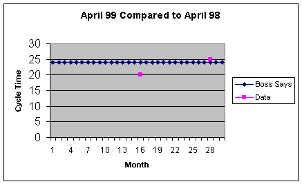
Figure 1.1.1 provides an example of a run chart tracking average monthly cycle times for materials coming into a manufacturing firm (this example is based on an actual experience I had in doing a logistics system analysis and design project for Johnson & Johnson's Sterile Design Company several years ago under a grant at the University of South Florida.) Cycle time is the elapsed time from when materials are ordered until they arrive. The average cycle time would be an average for all materials ordered in a particular month. So in April, 1998 (Month 16), the average cycle time was 20 days, or almost 3 weeks for all of the items ordered that month. Note the "Boss says" that no average monthly cycle time should be over 24 days, so that the April 1999 experience of 25 days produces an "Oh No" from the procurement office. At the minimum, these "Oh No's" require exception reports and create stress. In the worst cases, these "Oh No's" may lead to high turnover, a lot of sick leave, or "cover-up" responses, especially when team members believe the process is behaving as expected.

Figure 1.1.1

If the organization defines cycle time as an important output of the supply chain, then that variable should be measured. Such measurement enables the process to be analyzed so it can be improved, managed and controlled. Verifiable measurements, now often referred to as metrics (S. Melnyk, 1999), put data in its context and gives it meaning (D. Wheeler, 1993).

As we will learn in Modules 1.2 and 1.3 Notes, measurement of continuous numerical data such as time and dollars, involves measuring the center and spread or variability of the data. Once this is done, we can understand the "Voice of the Process," a term coined in 1924 by Walter Shewhart, one of the founding fathers of Statistical Process Control. 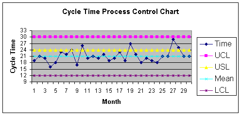So, rather than just looking at one data point in comparison to the bosses target, or just comparing a current data point to the same point a year ago, we analyze all 30 months of current cycle time data to discover the Voice of the Process in a Process Control Chart such as Figure 1.1.2.

Figure 1.1.2.

In Figure 1.1.2, the Voice of the Process suggests the process center or mean is 21 days over the past 30 months. Note that some of the monthly average observations are above the mean, and some are below - that is, there is deviation around the process mean. The maximum deviation for this process is computed as 30 days, and the minimum is 12. These are called the upper bound or upper control limit (UCL) of 30 and a lower control limit (LCL) of 12. These upper and lower limits are 9 days above and below the mean (we will see how to compute the mean and spread in Module 1.3.) For now, just accept the fact that any observation within the upper and lower control limit is called "noise." Every process generates noise when it is in control. Processes that are in control have the good properties of being stable and predictable. We will see how to construct these process control charts and control limits in Module 1.3 Notes.

Processes that are in control should not generate signals, or observations outside the control limits. Signals are also known as outliers. Whenever signals are encountered, such as a cycle time of 33 days, there should be an investigation to determine and correct the cause of the out-of-control problem.

The Voice of the Process helps us avoid the error of interpreting noise as if it were a signal - the first error in the interpretation of data. It also helps in avoiding the second error: failing to detect a signal when it is present (D. Wheeler, 1993). Note carefully that Figure 1.1.2 shows a process that is in control. Also note that the boss's specification limit of 24 days (referred to as "Boss Says" in Figure 1.1.1), is formally called an upper or lower specification limit, in the process control chart. As the chart shows, this process is not able to satisfy the boss 100 percent of the time as the boss's upper specification limit (USL) is within the upper control limit. Specification limits express the Voice of the Customer.

This is an important point. The proper translation of data into information gives us vital knowledge about the process. Even though the process is in control, the boss is unsatisfied. That is, being in control is not necessarily good or bad. "Goodness" or "badness" of a process depends on the targets set by the customer (here the boss would be an internal customer of the process - there are obviously both internal customers such as bosses and team workers, and external customers such as buyers of products and services.) A process that is in control is a good process if the customer's target specification limits are being met by the process. A process that is in control is a bad process if the customer's target specification limits are not being met by the process.

When the Voice of the Customer, expressed as target specification limits on the process, is not being met by the Voice of the Process, there is conflict. To resolve the conflict and satisfy the boss, we could reduce the variation of the process (make the upper and lower control limits "tighter"). For example, if the variation of the process were reduced to an UCL of 23 and a lower control limit of 19 around the current mean of 21, we would have an effective process with respect to the Voice of the Customer, since the boss's upper specification limit of 24 would be outside the upper control limit. This would mean there should never be an observation above 23. How can we reduce variation? One way would be to shift from common to dedicated carrier - the transportation cost is higher but the inventory carrying cost due to reduction in safety stock is much lower.

Another option is to shift the mean of the process, keeping the variation constant at plus or minus a total of 9 days. In this example, we would want to shift the mean from 21 to perhaps 14, which results in a new upper control limit of 23 days (14 plus 9). Here again, the upper control limit is lower than the customer's upper specification limit, so this process would be considered capable of meeting customer expectations. The mean could be shifted by switching to quicker, more costly modes of transportation. That cost was an accepted cost of the late 1980's and early 1990's as most companies began competing by both quality and cycle time reduction - getting product to market sooner, without defect.

A side note: please understand in this introductory example that our attention has been on the upper control limit and upper specification limit. This is common when cycle time is the variable of interest, since concern is usually with longer rather than shorter cycle times. Sometimes, we are interested in moving up lower control limits, such as when we are measuring profit contribution or revenue growth. Sometimes we are interested in both upper and lower control and specification limits such as in monitoring the tolerance of manufactured parts.

A third option is to reduce the variability and shift the mean - a combination approach. Here it is customary to reduce the variation before shifting the mean, since processes with little variation are much more stable. If the mean is shifted in a process with great variation, the shift may be undetectable.

Please note carefully that I omitted two other approaches that are, sadly, taken in many organizations. I say "sadly" since neither results in continuous improvement. One is for the "boss" (internal customer) to get angry with the team running the process and identify someone/some unit for punishment. In this example, this is virtually guaranteed since there are occasions in Figure 1.1.2 when the target specification limit is not met (there are observations above the upper specification limit of 24). Rather than getting angry with the team running the process, the boss should work with the team to improve the process (reduce variation or shift the mean), and provide the needed resources for the improvement.

Did you think of another approach that I omitted.....telling the customer ("boss" in this case) that he or she is wrong - the specification limit is too tight.....Hello.....!! In one of the first quality improvement seminars I was conducting for GE Client Business Services several years ago, I said; "to satisfy the customer when specification limits are within process control limits, reduce the variation, shift the mean, do both, or ask the customer to reset their specification limits." Well, there were about 40 students in the class and a strange hush fell upon the room.... the class leader finally said, "what, tell the customer they are wrong... not at GE!"

I agree with the GE philosophy, the customer is right. However, in my defense, I stated that the customer may have set unreasonable targets, at least in the short run. The Japanese auto manufacturers understood this many years ago when they started dealing with US vendors for auto parts. To get US vendors to deliver "zero-defect" parts and subassemblies would take a series of small continuous improvement steps (gradually setting tighter and tighter specification limits) to migrate from high percent defects to zero-defects. Of course the US vendors rapidly caught on when they realized that competition required high quality just for market entry - it wasn't a product differentiator any more.


I chose this example to illustrate that business statistics isn't about formulas to crank to turn in homework in college classes. Rather, it's about putting data in its context through appropriate measurement to understand and improve process capability and performance, and to make inferences and predictions. This course will hopefully expose you to that branch of decision sciences called statistics that enables us to put data in its context, and to transform that data into information and knowledge. Statistics enables managers to know how to (Leven, Berenson and Stephan, 1999):

Properly present and describe information (descriptive statistics)

Draw conclusions about populations based on information obtained from samples (inferential statistics)

Improve processes (Continuous Improvement)

Obtain reliable forecasts and predictions

The remainder of Module 1 will take us through descriptive and inferential statistics for continuous numerical variables such as time, whose data elements are measured in, for example, minutes or fractions of minutes. Other continuous variables include weight, measured in pounds or tons; height, measured in inches or feet; and revenue, variable cost or profit contribution measured in dollars or thousands of dollars. Discrete numerical data is distinguished from continuous numerical data in that the discrete number scale contains only discrete integers such as 1, 2, 3, as would be found in counting. For example, suppose there are 5 firms in a small data sample, and these firms make an average of $5,000 profit contribution. Here, the "5 firms" represent discrete data, and the "$5,000 profit" represents continuous data. Discrete data will be discussed in Module 5.

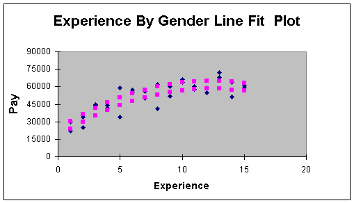
Modules 2 and 3 focus on regression and correlation analysis, or the study of the strength, form and direction of relationships between variables. In addition to understanding the relationship between variables, regression analysis is the tool managers use to make reliable predictions and forecasts. You may have read about female faculty members at the University of South Florida claiming gender bias in faculty salaries. A regression analysis of male versus female faculty salaries over time (the diamonds represent actual salaries and years of experience for a sample of male and female faculty members) quickly demonstrates the value of quantitative measurement in supporting a claim. Figure 1.1.3, although based on fictitious data, is representative of that analysis. This figure reflects that while both male (top curved prediction line of squares) and female (bottom curved prediction line of squares) faculty salaries increase at a decreasing rate (a common phenomenon at a university), males make more on average than females. In studies such as this, analysts need to take care that subjects are selected from similar disciplines and colleges to reduce the impact of confounding variables.

Figure 1.1.3.

In Module 5 we introduce categorical data-type variables that are measured by counting observations within a category level. For example, note in Figure 1.1.2 that four observations were above the upper specification limit. The boss would say we have four defects. In this scenario, the cycle time variable is considered a categorical variable with two values: late (cycle times above 24) and not late (cycle times at or below 24 days). The focus here is on the number of shipments that were defective (late), not the length of time they were late as in the continuous numerical variable example. Categorical variables then have named categories such as defective/not defective, in season/not in season, poor/satisfactory/good, and so forth. Much more on this subject when we get to Module 5.



References:

Anderson, D., Sweeney, D., & Williams, T. (2001). Contemporary Business Statistics with Microsoft Excel. Cincinnati, OH: South-Western, Chapter 1.

Leven, D., Berenson, M. & Stephan, D. (1999). Statistics for Managers Using Microsoft Excel (2nd ed.). Upper Saddle River, NJ: Prentice-Hall. Chapter 1.

Melnyk S. (March, 1999). "Metrics - The Missing Piece in Operations Management Research," Decision Line, Vol. 30, No. 2

Wheeler, D. (1993). Understanding Variation: The Key to Managing Chaos. Knoxville, TN: SPC Press, Inc.

About the Course

Module Schedule

Web Board