|
Module 1.1 Notes |
|
Index to Module One Notes
|
"If you know a thing only qualitatively, you know it no more than vaguely…If you know it quantitatively--grasping some numerical measure that distinguishes it from an infinite number of other possibilities--you are beginning to know it deeply…You comprehend some of its beauty and you gain access to its power and the understanding it provides…"
Carl Sagan (1997), "Billions and Billions: Thoughts on Life and Death At the Brink of the Millennium."
Let's move this thought into
a business world example to introduce statistics for managers. Don't worry about
how to do the computations - we will cover that later. For now, just focus on
the concepts illustrated in this introduction.
... If you don't know a process quantitatively, you run the risk of making at
least two errors (D. Wheeler, 1993).
The first error is to interpret noise as if it were a signal.
Figure 1.1.1 provides an example of a run chart tracking average monthly cycle
times for materials coming into a manufacturing firm (this example is based on
an actual experience I had in doing a logistics system analysis and design
project for Johnson & Johnson's Sterile Design Company several years ago
under a grant at the
Figure 1.1.1
If the organization defines cycle
time as an important output of the supply chain, then that variable should be
measured. Such measurement enables the process to be analyzed so it can be
improved, managed and controlled. Verifiable measurements, now often referred
to as metrics (S. Melnyk, 1999), put data in its context and gives it meaning
(D. Wheeler, 1993).
As we will learn in Modules 1.2 and 1.3 Notes, measurement of continuous
numerical data such as time and dollars, involves measuring the center and
spread or variability of the data. Once this is done, we can understand the "Voice
of the Process," a term coined in 1924 by Walter Shewhart, one of the
founding fathers of Statistical Process Control. So, rather than just looking
at one data point in comparison to the bosses target, or just comparing a
current data point to the same point a year ago, we analyze all 30 months of
current cycle time data to discover the Voice of the Process in a Process
Control Chart such as Figure 1.1.2.
Figure 1.1.2.
In Figure 1.1.2, the Voice of the Process suggests the process center or mean
is 21 days over the past 30 months. Note that some of the monthly average
observations are above the mean, and some are below - that is, there is deviation
around the process mean. The maximum deviation for this process is computed as
30 days, and the minimum is 12. These are called the upper bound or upper
control limit (UCL) of 30 and a lower control limit (LCL) of
12. These upper and lower limits are 9 days above and below the mean (we will
see how to compute the mean and spread in Module 1.3.) For now, just accept the
fact that any observation within the upper and lower control limit is called
"noise." Every process generates noise when it is in control.
Processes that are in control have the good properties of being stable and
predictable. We will see how to construct these process control charts and
control limits in Module 1.3 Notes.
Processes that are in control should not generate signals, or
observations outside the control limits. Signals are also known as outliers.
Whenever signals are encountered, such as a cycle time of 33 days, there should
be an investigation to determine and correct the cause of the out-of-control
problem.
The Voice of the Process helps us avoid the error of interpreting noise as if
it were a signal - the first error in the interpretation of data. It also helps
in avoiding the second error: failing to detect a signal when it is present (D.
Wheeler, 1993). Note carefully that Figure 1.1.2 shows a process that is in
control. Also note that the boss's specification limit of 24 days (referred to
as "Boss Says" in Figure 1.1.1), is formally called an upper or
lower specification limit, in the process control chart. As the chart
shows, this process is not able to satisfy the boss 100 percent of the time as
the boss's upper specification limit (USL) is within the upper control limit.
Specification limits express the Voice of the Customer.
This is an important point. The proper translation of data into information
gives us vital knowledge about the process. Even though the process is in
control, the boss is unsatisfied. That is, being in control is not necessarily
good or bad. "Goodness" or "badness" of a process depends
on the targets set by the customer (here the boss would be an internal customer
of the process - there are obviously both internal customers such as bosses and
team workers, and external customers such as buyers of products and services.)
A process that is in control is a good process if the customer's target
specification limits are being met by the process. A process that is in control
is a bad process if the customer's target specification limits are not being
met by the process.
When the Voice of the Customer, expressed as target specification limits
on the process, is not being met by the Voice of the Process, there is
conflict. To resolve the conflict and satisfy the boss, we could reduce the
variation of the process (make the upper and lower control limits
"tighter"). For example, if the variation of the process were reduced
to an UCL of 23 and a lower control limit of 19 around the current mean of 21,
we would have an effective process with respect to the Voice of the
Customer, since the boss's upper specification limit of 24 would be outside
the upper control limit. This would mean there should never be an observation
above 23. How can we reduce variation? One way would be to shift from common to
dedicated carrier - the transportation cost is higher but the inventory
carrying cost due to reduction in safety stock is much lower.
Another option is to shift the mean of the process, keeping the
variation constant at plus or minus a total of 9 days. In this example, we
would want to shift the mean from 21 to perhaps 14, which results in a new
upper control limit of 23 days (14 plus 9). Here again, the upper control limit
is lower than the customer's upper specification limit, so this process would
be considered capable of meeting customer expectations. The mean could be
shifted by switching to quicker, more costly modes of transportation. That cost
was an accepted cost of the late 1980's and early 1990's as most companies
began competing by both quality and cycle time reduction - getting product to
market sooner, without defect.
A side note: please understand in this introductory example that our attention
has been on the upper control limit and upper specification limit. This is
common when cycle time is the variable of interest, since concern is usually
with longer rather than shorter cycle times. Sometimes, we are interested in
moving up lower control limits, such as when we are measuring profit
contribution or revenue growth. Sometimes we are interested in both upper and
lower control and specification limits such as in monitoring the tolerance of
manufactured parts.
A third option is to reduce the variability and shift the mean - a
combination approach. Here it is customary to reduce the variation before
shifting the mean, since processes with little variation are much more stable.
If the mean is shifted in a process with great variation, the shift may be
undetectable.
Please note carefully that I omitted two other approaches that are, sadly,
taken in many organizations. I say "sadly" since neither results in
continuous improvement. One is for the "boss" (internal customer) to
get angry with the team running the process and identify someone/some unit for
punishment. In this example, this is virtually guaranteed since there are
occasions in Figure 1.1.2 when the target specification limit is not met (there
are observations above the upper specification limit of 24). Rather than
getting angry with the team running the process, the boss should work with the
team to improve the process (reduce variation or shift the mean), and provide
the needed resources for the improvement.
Did you think of another approach that I omitted.....telling the customer
("boss" in this case) that he or she is wrong - the specification
limit is too tight.....Hello.....!! In one of the first quality improvement
seminars I was conducting for GE Client Business Services several years ago, I
said; "to satisfy the customer when specification limits are within
process control limits, reduce the variation, shift the mean, do both, or ask the
customer to reset their specification limits." Well, there were about 40
students in the class and a strange hush fell upon the room.... the class
leader finally said, "what, tell the customer they are wrong... not at
GE!"
I agree with the GE philosophy, the customer is right. However, in my defense,
I stated that the customer may have set unreasonable targets, at least in the
short run. The Japanese auto manufacturers understood this many years ago when
they started dealing with US vendors for auto parts. To get US vendors to
deliver "zero-defect" parts and subassemblies would take a series of
small continuous improvement steps (gradually setting tighter and tighter
specification limits) to migrate from high percent defects to zero-defects. Of
course the
I chose this example to illustrate that business statistics isn't about
formulas to crank to turn in homework in college classes. Rather, it's about
putting data in its context through appropriate measurement to understand and
improve process capability and performance, and to make inferences and
predictions. This course will hopefully expose you to that branch of decision
sciences called statistics that enables us to put data in its context, and to
transform that data into information and knowledge. Statistics enables managers
to know how to (Leven, Berenson and Stephan, 1999):
![]() Properly present and describe
information (descriptive statistics)
Properly present and describe
information (descriptive statistics)
![]() Draw
conclusions about populations based on information obtained from samples (inferential
statistics)
Draw
conclusions about populations based on information obtained from samples (inferential
statistics)
![]() Improve
processes (Continuous Improvement)
Improve
processes (Continuous Improvement)
![]() Obtain
reliable forecasts and predictions
Obtain
reliable forecasts and predictions
The remainder of Module 1
will take us through descriptive and inferential statistics for continuous
numerical variables such as time, whose data elements are measured in, for
example, minutes or fractions of minutes. Other continuous variables include
weight, measured in pounds or tons; height, measured in inches or feet; and revenue,
variable cost or profit contribution measured in dollars or thousands of
dollars. Discrete numerical data is distinguished from continuous numerical
data in that the discrete number scale contains only discrete integers such as
1, 2, 3, as would be found in counting. For example, suppose there are 5 firms
in a small data sample, and these firms make an average of $5,000 profit
contribution. Here, the "5 firms" represent discrete data, and the
"$5,000 profit" represents continuous data. Discrete data will be
discussed in Module 5.
Modules 2 and 3 focus on regression and correlation analysis, or the study of
the strength, form and direction of relationships between variables. In
addition to understanding the relationship between variables, regression analysis
is the tool managers use to make reliable predictions and forecasts. You may
have read about female faculty members at the
Figure 1.1.3.
In Module 5 we
introduce categorical data-type variables that are measured by counting
observations within a category level. For example, note in Figure 1.1.2 that
four observations were above the upper specification limit. The boss would say
we have four defects. In this scenario, the cycle time variable is considered a
categorical variable with two values: late (cycle times above 24) and not late
(cycle times at or below 24 days). The focus here is on the number of shipments
that were defective (late), not the length of time they were late as in the
continuous numerical variable example. Categorical variables then have named
categories such as defective/not defective, in season/not in season,
poor/satisfactory/good, and so forth. Much more on this subject when we get to
Module 5.
Sampling
Concepts & Procedures
In business,
data usually arises from accounting transactions or management processes (i.e.,
inventory, sales, and payroll). Much of the data we analyze were recorded
without explicit consideration, yet many decisions may depend on the data. Let's go over some important definitions
before you collect the data for your assignments.
A subject
or individual is a single member of a collection of items that we want to
study. A variable is a
characteristic of a subject or individual such as employee’s income or invoice
amount. A data set consists of all
the values of all the variables for all the individuals we have chosen to observe,
that is, a collection of observations. Table 1.1 relates the type of dataset
with the amount of variables you may want to study/present. In Asgn 1, for
example, will conduct a univariate study; that is, we are interested in
describing a process/construct through only one variable or characteristic
process. In my example for Module 1, I
am interested in measuring customer service which of course is composed
of many variables/characteristics (reliability, on time delivery, etc). However, I elected to present/describe it
only in terms of cycle time, which is viewed by management as very
important to please our customers. Therefore, in Module 1, we'll deal with
univariate study.
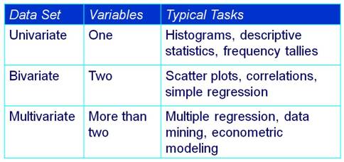
Table 1.1
Modules 2
will study Bivariate data through simple regression analysis. Modules 3, 4, and
5 will require the use of multivariate dataset.
Figure 1.1.4 illustrate a multivariate data set.
Figure 1.1.4
Sample or Census?
A sample
involves looking only at some items selected from the population. A census is an
examination of all items in a defined population. Why can’t the United States Census survey
every person in the population?
Situations
Where a Sample May Be Preferred …
·
Infinite
Population: No census is possible if the
population is infinite or of indefinite size (an assembly line can keep
producing bolts, a doctor can keep seeing more patients).
·
Destructive
Testing: The act of sampling may destroy or
devalue the item (measuring battery life, testing auto crashworthiness, or
testing aircraft turbofan engine life).
·
Timely
Results: Sampling may yield more timely results
than a census (checking wheat samples for moisture and protein content,
checking peanut butter for aflatoxin contamination).
·
Accuracy: Sample
estimates can be more accurate than a census.
Instead of spreading limited resources thinly to attempt a census, our
budget of time and money might be better spent to hire experienced staff,
improve training of field interviewers, and improve data safeguards.
·
Cost:
Even if it is
feasible to take a census, the cost, either in time or money, may exceed our
budget.
·
Sensitive
Information: Some
kinds of information are better captured by a well-designed sample, rather than
attempting a census. Confidentiality may also be improved in a carefully-done
sample.
Situations
Where a Census May Be Preferred …
·
Small
Population: If the
population is small, there is little reason to sample, for the effort of data
collection may be only a small part of the total cost.
·
Large
Sample Size: If the
required sample size approaches the population size, we might as well go ahead
and take a census.
·
Database
Exists: If the data
are on disk we can examine 100% of the cases.
But auditing or validating data against physical records may raise the
cost.
·
Legal
Requirements: Banks
must count all the cash in bank teller drawers at the end of each
business day. The U.S. Congress forbade
sampling in the 2000 decennial population census.
Pause and reflect: A parameter is any measurement that
describes an entire population. Usually, the parameter value is unknown since
we rarely can observe the entire population.
Parameters are often (but not always) represented by Greek letters
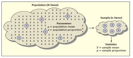
Figure 1.1.5
Statistics
are any measurement computed from a sample. Usually, the statistic is regarded as an
estimate of a population parameter.
Sample statistics are often (but not always) represented by Roman
letters.
Let's review two situations in which samples provide estimates of population
parameters.
1. a tire manufacturer developed a new tire designed to provide an
increase in mileage over the firm's current line of tires. To estimate the mean
number of miles provided by the new tire, the manufacturer selected a sample of
120 new tires for testing. The test provided a sample mean of 36,500 miles.
Hence, an estimate of the mean tire mileage for the population of new tires was
36,500 miles
2. Members of a political party were considering supporting a particular
candidate for election to the U.S. Senate, and party leaders wanted an estimate
of the proportion of registered voters supporting the candidate. The time and
cost associated with contacting every potential voter were prohibitive. Hence,
a sample of 400 registered voters was selected and 160 of the 400 voters
indicated a preference for the candidate.
An estimaete of the proportion of the population of registered voters
supporting the candidate was 160/400 = 0.40.
These two examples illustrate why samples are used. It is important to
realize that sample results provide only estimates of the value of the
population characteristics. We do not expect the mean mileage for all tires in
the population to be exactly 36,500 miles, nor do we expect exactly 0.40, or
40%, of the population of registered voters to support the candidate. However,
proper sampling methods, the sample results will provide 'good' estimates of
the population parameters. Let's briefly
see some types of sampling procedures.
Sampling procedures:
·
Simple
Random Sample: Use random numbers to select items from a
list (e.g., VISA cardholders).
·
Systematic
Sample: Select every kth
item from a list or sequence (e.g., restaurant customers).
·
Stratified
Sample: Select
randomly within defined strata (e.g., by age, occupation, gender).
·
Cluster
Sample: Like
stratified sampling except strata are geographical areas (e.g., zip codes).
·
Judgment
Sample : Use expert
knowledge to choose “typical” items (e.g., which employees to interview).
·
Convenience
Sample : Use a sample
that happens to be available (e.g., ask co-worker opinions at lunch).
·
Focus
Groups : In-depth
dialog with a representative panel of individuals (e.g. iPod users).
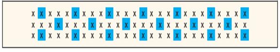
A very
important sampling procedure is called Simple Random Sampling: Every item in the population
of N items has the same chance of being chosen in the sample of n items. We rely on random numbers to
select a name.
Example:


Figure 1.1.6
There are 48 names
in the list presented in figure 1.1.6 and we need to select one at random. There are random tables we could use for this
task but in this course we'll use Excel random number generator. In Excel, type in a cell,
=RANDBETWEEN(1,48). The formula returns
a random number between 1 and 48. In the
example above, the return is 44, so we can select Stephanie from the list. When
the data is arranged in a rectangular array (or Table), an item can be
chosen at random by randomly selecting a row and column.
Use
=RANDBETWEEN(1,3) function to randomly choose a column and
=RANDBEWTEEN(1,4) to choose a row.
This way, each item has an equal chance of being selected.
Often, we
have the need to randomize a LIST: In
Excel, use function =RAND() beside each row to create a column of random
numbers between 0 and 1. Let's see an example.
|
Name |
Major |
Gender |
|
|
Claudia |
Accounting |
F |
|
|
Dan |
Economics |
M |
|
|
Dave |
Human Res |
M |
|
|
Kalisha |
MIS |
F |
|
|
LaDonna |
Finance |
F |
|
|
Marcia |
Accounting |
F |
|
|
Matt |
Undecided |
M |
|
|
Moira |
Accounting |
F |
|
|
Rachel |
Oper Mgt |
F |
|
|
Ryan |
MIS |
M |
|
|
Tammy |
Marketing |
F |
|
|
Victor |
Marketing |
M |
|
|
Rand |
Name |
Major |
Gender |
|
0,382091 |
Claudia |
Accounting |
F |
|
0,730061 |
Dan |
Economics |
M |
|
0,143539 |
Dave |
Human Res |
M |
|
0,906060 |
Kalisha |
MIS |
F |
|
0,624378 |
LaDonna |
Finance |
F |
|
0,229854 |
Marcia |
Accounting |
F |
|
0,604377 |
Matt |
Undecided |
M |
|
0,798923 |
Moira |
Accounting |
F |
|
0,431740 |
Rachel |
Oper Mgt |
F |
|
0,334449 |
Ryan |
MIS |
M |
|
0,836594 |
Tammy |
Marketing |
F |
|
0,402726 |
Victor |
Marketing |
M |
Now you sort
from in ascending order. The first n
items are a random sample of the entire list (they are as likely as any
others).
|
Rand |
Name |
Major |
Gender |
|
0,143539 |
Dave |
Human Res |
M |
|
0,229854 |
Marcia |
Accounting |
F |
|
0,334449 |
Ryan |
MIS |
M |
|
0,382091 |
Claudia |
Accounting |
F |
|
0,402726 |
Victor |
Marketing |
M |
|
0,431740 |
Rachel |
Oper Mgt |
F |
|
0,604377 |
Matt |
Undecided |
M |
|
0,624378 |
LaDonna |
Finance |
F |
|
0,730061 |
Dan |
Economics |
M |
|
0,798923 |
Moira |
Accounting |
F |
|
0,836594 |
Tammy |
Marketing |
F |
|
0,906060 |
Kalisha |
MIS |
F |
Systematic
Sampling: Sample by choosing every kth item
from a list, starting from a randomly chosen entry on the list. Systematic
sampling should yield acceptable results unless patterns in the population happen
to recur at periodicity k. It can
be used with unlistable or infinite populations. Systematic samples are well-suited to
linearly organized physical populations.
A systematic sample of n items from a population of N items
requires that periodicity k be approximately N/n. For
example, out of 501 companies, we want to obtain a sample of 25. What should
the periodicity k be? k = N/n , 501/25 » 20. So,
we should choose every 20th company from a random starting point.
For example, starting at item 2, we sample every k = 4 items to
obtain a sample of n = 20 items from a list of N = 78 items.
Note that N/n = 78/20 » 4.
That is all for now folks. Try to
apply some of these concepts when considering your data for the assignments in
this course. Remember that a good
sampling procedure helps eliminate bias and increase the chance of a good
estimate of the population parameter. We'll see more about sampling when we get
to module 5.
-x-x-x-x-x-x-
References:
D.
D. Groebner, P. Shannon, P.
Fry & K. Smith. Business Statistics:
A Decision Making Approach, Seventh Edition, Prentice Hall, Chapter 1,
18
Ken
Black. Business Statistics for Contemporary Decision Making. Fourth Edition,
Wiley. Chapter 18
Leven, D., Berenson, M. &
Stephan, D. (1999). Statistics for Managers Using Microsoft Excel (2nd ed.).
Melnyk S. (March, 1999). "Metrics - The Missing Piece in Operations
Management Research," Decision Line, Vol. 30, No. 2
Wheeler, D. (1993).
Understanding Variation: The Key to Managing Chaos.
| Return to Module 1 Overview | Return to top of page |