Fore….an ancient term of warning bearing the threat of harm at worst, and uncertainty at best, to those within potential range...

+ Cast… serving up a projectile to the unseen and usually unknown beneath the deceptive surface

= Forecast.... a warning to those who use it... a confession of uncertainty (or deception) by those who create it... a threat of harm to those in its path

From Tom Brown in Getting the Most of Forecasting

 2.1: Introduction to Forecasting

Although the quantitative methods of business can be studied as independent modules, I believe it is appropriate that the text places the forecasting material right after decision analysis. Recall in our decision analysis problems, the states of nature generally referred to varying levels of demand or some other unknown variable in the future. Predicting, with some measure of accuracy or reliability, what those levels of demand will be is our next subject.

Forecasts are more than simple extrapolations of past data into the future using mathematical formulas, or gathering trends from experts…. Forecasts are mechanisms of arriving at measures for planning the future. When done correctly, they provide an audit trail and a measure of their accuracy. When not done correctly, they remind us of Tom Brown's clever breakdown of the term repeated at the opening of these notes.

Not only do forecasts help us plan, they help us save money! I am aware of one company that reduced its investment in inventory from $ 28 million to $22 million by adopting a formal forecasting method that reduced forecast error by 10%. This is an example of forecasts helping product companies replace inventory with information, which not only saves money but improves customer response and service.

When we use the term "forecasting" in a quantitative methods course, we are generally referring to quantitative time series forecasting methods. These models are appropriate when: 1) past information about the variable being forecast is available, 2) the information can be quantified, and 3) it is assumed that patterns in the historical data will continue into the future. If the historical data is restricted to past values of the response variable of interest, the forecasting procedure is called a time series method.

For example, many sales forecasts rely on the classic time series methods that we will cover in this module. When the forecast is based on past sales, we have a time series forecast. A side note: although I said "sales" above, whenever possible, we try to forecast sales based on past demand rather than sales… why? Suppose you own a T-shirt shop at the beach. You stock 100 "Spring Break 2000" T-shirts getting ready for Spring Break. Further suppose that 110 Spring Breakers enter your store to buy Spring Break 2000 T-shirts. What are your sales? That's right, 100. But what is your demand? Right again, 110. You would want to use the demand figure, rather than the sales figure, in preparing for next year as the sales figures do not capture your stock outs. So why do many companies make sales forecasts based on past sales and not demand? The chief reason is cost - sales are easily captured at the check out station, but you need some additional feature on your management information system to capture demand.

Back to the introduction. The other major category of forecasting methods that rely on past data are regression models, often referred to as "causal" models as in our text. These models base their prediction of future values of the response variable, sales for example, on related variables such as disposable personal income, gender, and maybe age of the consumer. You studied regression models in the statistics course, so we will not cover them in this course. However, I do want to say that we should use the term "causal" with caution, as age, gender, or disposable personal income may be highly related to sales, but age, gender or disposable personal income may not cause sales. We can only prove causation in an experiment.

The final major category of forecasting models includes qualitative methods which generally involve the use of expert judgment to develop the forecast. These methods are useful when we do not have historical data, such as the case when we are launching a new product line without past experience. These methods are also useful when we are making projections into the far distant future. We will cover one of the qualitative models in this introduction.

First, lets examine a simple classification scheme for general guidelines in selecting a forecasting method, and then cover some basic principles of forecasting.


Selecting a Forecasting Method

The following table illustrates general guidelines for selecting a forecasting method based on time span and purpose criteria.

Table 2.1.1

Time Span	Purpose	Forecasting Method
Long Range (3 or more years)	Capital Budgets Product Selection Plant Location	Delphi Expert Judgment Sales Force Composite
Intermediate (1 to 3 years)	Capacity Planning Sales Planning	Regression Time Series Decomposition
Short Range (1 year or less)	Sales Forecasting Scheduling Inventory Control	Trend Projection Moving Average Exponential Smoothing

Please understand that these are general guidelines. You may find a company using trend projection to make reliable forecasts for product sales 3 years into the future. It should also be noted that since companies use computer software time series forecasting packages rather than hand computations, they may try several different techniques and select the technique which has the best measure of accuracy (lowest error).

As we discuss the various techniques, and their properties, assumptions and limitations, I hope that you will gain an appreciation for the above classification scheme.

Forecasting Principles
Classification schemes such as the one above are useful in helping select forecasting methods appropriate to the time span and purpose at hand. There are also some general principles that should be considered when we prepare and use forecasts, especially those based on time series methods.

Oliver W. Wight in Production and Inventory Control in the Computer Age*, and Thomas H. Fuller in Microcomputers in Production and Inventory Management** developed a set of principles for the production and inventory control community a while back that I believe have universal application.

1. Unless the method is 100% accurate, it must be simple enough so people who use it know how to use it intelligently (understand it, explain it, and replicate it)*.

2. Every forecast should be accompanied by an estimate of the error (the measure of its accuracy).*

3. Long term forecasts should cover the largest possible group of items; restrict individual item forecasts to the short term.**

4. The most important element of any forecast scheme is that thing between the keyboard and the chair.**

The first principle suggests that you can get by with treating a forecast method as a "black box," as long as it is 100% accurate. That is, if an analyst simply feeds historical data into the computer and accepts and implements the forecast output without any idea how the computations were made, that analyst is treating the forecast method as a black box. This is ok as long as the forecast error (actual observation - forecast observation) is zero. If the forecast is not reliable (high error), the analyst should be, at least, highly embarrassed by not being able to explain what went wrong. There may be much worse ramifications than embarrassment if budgets and other planning events relied heavily on the erroneous forecast.

The second principle is really important. In section 2.2 we will introduce a simple way to measure forecast error, the difference between what actually occurs and what was predicted to occur for each forecast time period. Here is the idea. Suppose an auto company predicts sales of 30 cars next month using Method A. Method B also comes up with a prediction of 30 cars. Without knowing the measure of accuracy of the two Methods, we would be indifferent as to their selection. However, if we knew that the composite error for Method A is +/- 2 cars over a relevant time horizon; and the composite error for Method B is +/- 10 cars, we would definitely select Method A over Method B.

Why would one method have so much error compared to another? That will be one of our learning objectives in this module. It may be because we used a smoothing method rather than a method that incorporates trend projection when we should not have - such as when the data exhibits a growth trend. Smoothing methods such as exponential smoothing, always lag trends which results in forecast error.

The third principle might best be illustrated by an example. Suppose you are Director of Operations for a hospital, and you are responsible for forecasting demand for patient beds. If your forecast was going to be for capacity planning three years from now, you might want to forecast total patient beds for the year 2003. On the other hand, if you were going to forecast demand for patient beds for April 2000, for scheduling purposes, then you would need to make separate forecasts for emergency room patient beds, surgery recovery patient beds, OB patient beds, and so forth. When much detail is required, stick to a short term forecast horizon; aggregate your product lines/type of patients/etc. when making long term forecasts. This generally reduces the forecast error in both situations.

We should apply the last principle to any quantitative method. There is always room for judgmental adjustments to our quantitative forecasts. I like this quote from Alfred North Whitehead in An Introduction to Mathematics, 1911:

"[T]here is no more common error than to assume that, because prolonged and accurate mathematical calculations have been made, the application of the result to some fact of nature is absolutely certain."

Of course, judgment can be off too. How about this forecast made in 1943 by IBM Chairman Thomas Watson:

"I think there's a world market for about five computers."

How can we improve the application of judgment? That is our next subject.


The Delphi Method of Forecasting
The Delphi Method of forecasting is a qualitative technique made popular by the Rand Corporation. It belongs to the family of techniques that include methods such as Grass Roots, Market Research Panel, Historical Analogy, Expert Judgment, and Sales Force Composite. The thing in common with these approaches is the use of the opinions of experts, rather than historical data, to make predictions and forecasts. The subjects of these forecasts are typically the prediction of political, social, economic or technological developments that might suggest new programs, products, or responses from the organization sponsoring the Delphi study.

My first experience with expert judgment forecasting techniques was at my last assignment during my past career in the United States Air Force. In that assignment, I was Director of Transportation Programs at the Pentagon. Once a year, my boss, the Director of Transportation, would gather senior leadership (and their action officers) at a conference to formulate transportation plans and programs for the next five years. These programs then became the basis for budgeting, procurement, and so forth. One of the exercises we did was a Delphi Method to predict developments that would have significant impact on Air Force Transportation programs. I recall one of the developments we predicted at a conference in the early 1980's was the accelerated movement from decentralized to centralized strategic transportation systems in the military. As a result, we began to posture the Air Force for the unified transportation command several years before it became a reality.

Step 1. The Delphi Method of Forecasting, like the other judgment techniques, begins with selecting the experts. Of course, this is where these techniques can fail - when the experts are really not experts at all. Maybe the boss is included as an "expert" for the Delphi study, but while the boss is great at managing resources, he or she may be terrible at reading the environment and predicting developments.

Step 2. The first formal step is to obtain an anonymous forecast on the topic of interest. This is called Round 1. Here, the experts would be asked to provide a political, economic, social or technological developments of interest to the organization sponsoring the Delphi Method.

The anonymous forecasts may be gathered through a Web Site, via e-mail or by questionnaire. They may also be gathered in a live group setting but the "halo effect" may stifle the free flow of the predictions. For example, it would be common for the group of experts gathered at the Pentagon to include general officers. Several of the generals were great leaders in the field, but not great visionaries when it came to logistics developments. On the other hand, their lieutenant colonel action officers were very good thinkers and knew much about what was on the horizon for logistics and transportation systems. However, because of the classic respect for rank, the younger officers might not have been forthcoming if we did not use an anonymous method to get the first round of forecasts.

Step 3. The third step in the Delphi Method involves the group facilitator summarizing and redistributing the results of the Round One forecasts. This is typically a "laundry list" of developments. The experts are then asked to respond to the Round One "laundry list" by indicating the year in which they believed the development would occur; or to state this development will "never occur." This is called Round 2.

Step 4. The fourth step, Round 3, involves the group facilitator summarizing and redistributing the results of the Round Two. This includes a simple statistical display, typically the median and interquartile range, for the data (years a development will occur) from Round 2. The summary would also include the percent of experts reporting "never occur" for a particular development. In this Round, the experts are asked to modify, if they wish, their predictions. The experts are also given the opportunity to provide arguments challenging or supporting the "never occur" predictions for a particular development, and to challenge or support the years outside the interquartile range.

Step 5. The fifth step, Round 4, repeats Round 3 - the experts receive a new statistical display with arguments - and are requested to provide new forecasts and/or counter arguments.

Step 6. Round 4 is repeated until consensus is formed, or at least, a relatively narrow spread of opinions. My experience is that by Round 4, we had a good idea of the developments we should be focusing upon.

If the original objective of the Delphi Method is to produce a number rather than a development trend, then Round 1 simply asks the experts for their first prediction. This might be to predict product demand for a new product line for a consumer products company or to predict the DJIA one year out for a mutual fund company managing a blue chip index fund.

Let's do a "for fun" (not graded and purely volunteer) Delphi Exercise. Suppose you are a market expert and wish to join the other experts in our class in predicting what the DJIA will be on April 16, 2001 (as close to tax due date as possible). I will post a Conference Topic called "DJIA Predictions" on the course Web Board, within the Module 2 conference. Please reply to that conference topic by simply stating what you think the DJIA will close at on April 16, 2001. Please respond by January 27, 2001, so I can post the summary statistics before we leave the forecasting material on February 3rd.

We will now begin our discussion of quantitative time series forecasting methods.


2.2: Smoothing Methods

In this section we want to cover the components of a time series; naive, moving average and exponential smoothing methods of forecasting; and measuring forecast accuracy for each of the methods introduced.

Pause and Reflect
Recall that there are three general classes of forecasting or prediction models. Qualitative methods, including the Delphi, rely on expert judgment and opinion, not historical data. Regression models rely on historical information about both predictor variables and the response variable of interest. Quantitative time series forecasting methods rely on historical numerical information about the variable of interest and assume patterns in the past will continue into the future. This section begins our study of the time series models, beginning with patterns or components of time series.

Components of a Time Series
The patterns that we may find in a time series of historical data include the average, trend, seasonal, cyclical and irregular components. The average is simply the mean of the historical data. Trend describes real growth or decline in average demand or other variable of interest, and represents a shift in the average.

The seasonal component reflects a pattern that repeats within the total time frame of interest. For example, 15 years ago in Southwest Florida, airline traffic was much higher in January - April, peaking in March. October was the low month. This seasonal pattern repeated through 1988. Between 1988 and 1992, January - April continued to repeat each year as high months, but the peaks were not as high as before, nor the off-season valleys as low as before, much to the delight of the hotel and tourism industries. The point is, seasonal peaks repeat within the time frame of interest - usually monthly or quarterly seasons within a year, although there can be daily seasonality in the stock market (Mondays and Fridays showing higher closing averages than Tuesdays - Thursdays) as an example.

The cyclical component shows recurring values of the variable of interest above or below the average or long-run trend line over a multiyear planning horizon. The length of cycles is not constant, as with the length of seasonal peaks and valleys, making economic cycles much tougher to predict. Since the patterns are not constant, multiple variable models such as econometric and multiple regression models are better suited to predict cyclical turning points than time series models.

The last component is what's left! The irregular component is the random variation in demand that is unexplained by the average, trend, seasonal and/or cyclical components of a time series. As in regression models, we try to make the random variation as low as possible.

Quantitative models are designed to address the various components covered above. Obviously, the trend projection technique will work best with time series that exhibit an historical trend pattern. Time series decomposition, which decomposes the trend and seasonal components of a time series, works best with times series having trend and seasonal patterns. Where does that leave our first set of techniques, smoothing methods? Actually, smoothing methods work well in the presence of average and irregular components. We start with them next.

Before we start, lets get some data. This time series consists of quarterly demand for a product. Historical data is available for 12 quarters, or three years. Table 2.2.1 provides the history.

Table 2.2.1

Time	Quarter	Actual Demand
1	1	398
2	2	395
3	3	361
4	4	400
5	1	410
6	2	402
7	3	378
8	4	440
9	1	465
10	2	460
11	3	430
12	4	473
13	1
14	2
15	3
16	4

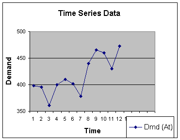
Figure 2.2.1 provides a graph of the time series. This graph was prepared in Excel using the Chart Wizard's Line Plot chart assistant. It is not important what software is used to graph the historical time series - but it is important to "look at" the data. Even making a pen and paper sketch is useful to get a "feel" for the data, and see if there might be trend and/or seasonal components in the time series.

Figure 2.2.1




Moving Average Method
A simple technique which works well with data that has no trend, seasonality nor cyclic components is the moving average method. Admittedly, this example data set has trend (note the overall growth rate from period 1 to 12), and seasonality (note that every third quarter reflects a decrease in historical demand). But let's apply the moving average technique to this data so we will have a basis for comparison with other methods later on.

A three period moving average forecast is a method that takes three periods of data and creates an average. That average is the forecast for the next period. For this data set, the first forecast we can compute is for Period 4, using actual historical data from Periods 1, 2 and 3 (since its a three period moving average). Then, after Period 4 occurs, we can make a forecast for Period 5, using historical data from Periods 2, 3, and 4. Note that Period 1 dropped off, hence the term moving average. This technique then assumes that actual historical data in the far distant past, is not as useful as more current historical data in making forecasts.

Before showing the formulas and illustrating this example, let me introduce some symbols. In this module, I will be using the symbol F_t to represent a forecast for period t. Thus, the forecast for period 4 would be shown as F₄. I will use the symbol Y_t to represent the actual historical value of the variable of interest, such as demand, in period t. Thus, the actual demand for period 1 would be shown as Y₁.

Now to carry forward the computations for a three period moving average. The forecast for period four is:

F₄ = (Y₁ + Y₂ + Y₃) / 3 = (398 + 395 + 361) / 3 = 384.7

To generate the forecast for period five:

F₅ = (Y₂ + Y₃ + Y₄) / 3 = (395 + 361 + 400) / 3 = 385.3

We continue through the historical data until we get to the end of Period 12 and make our forecast for Period 13 based on actual demand from Periods 10, 11 and 12. Since Period 12 is the last period for which we have data, this ends our computations. If someone was interested in making a forecast for Periods 14, 15, and 16, as well as Period 13, the best that could be done with the moving average method would be to make the "out period" forecasts the same as the most current forecast. This is true because moving average methods cannot grow or respond to trend. This is the chief reason these types of methods are limited to short term applications, such as what is the demand for the next period.

The forecast calculations are summarized in Table 2.2.2.

Table 2.2.2

Time	Quarter	Actual Demand (Yt)	Forecast (Ft)
1	1	398
2	2	395
3	3	361
4	4	400	384.7
5	1	410	385.3
6	2	402	390.3
7	3	378	404.0
8	4	440	397.6
9	1	465	406.7
10	2	460	427.7
11	3	430	455.0
12	4	473	451.7
13	1		454.3
14	2		454.3
15	3		454.3
16	4		454.3

Thus finishes our first time series forecast...but wait a minute...is it any good? To answer that question, we need to measure the accuracy of the forecast. Then, for all other forecasts presented, we will include that method's measure of accuracy.

Measuring the Error: Forecast Accuracy
The criteria for selecting between forecasting models, and for keeping tabs of how well a forecast is doing once it is implemented is called measuring the accuracy or the error of the forecast. To do this, we simply have to compute the average error of a forecast over an appropriate period of time. Typically, the appropriate period of time would be the period of time from which data was gathered and forecasts were applied.
Forecast error in time period t (E_t) is the actual value of the time series minus the forecasted value in time period y.

Error in time t = E_t = ( Y_t - F_t )

Table 2.2.3 illustrates the error computations for the three period moving average model.

Table 2.2.3

Time	Quarter	Actual Demand (Yt)	Forecast (Ft)	Error (Et)	Error2 (Et2)
1	1	398
2	2	395
3	3	361
4	4	400	384.7	15.3	235.1
5	1	410	385.3	24.7	608.4
6	2	402	390.3	11.7	136.1
7	3	378	404.0	-26.0	676.0
8	4	440	397.6	43.3	1877.8
9	1	465	406.7	58.3	3402.8
10	2	460	427.7	32.3	1045.4
11	3	430	455.0	-25.0	625
12	4	473	451.7	21.3	455.1
13	1		454.3
14	2		454.3
15	3		454.3
16	4		454.3
				SSE	9061.78
				MSE	1006.86
				RMSE	31.73

Since we are interested in measuring the magnitude of the error to determine forecast accuracy, note that I square the error to remove the plus and minus signs. Then, we simple average the squared errors. To compute an average or a mean, first sum the squared errors (SSE), then divide by the number of errors to get the mean squared error (MSE), then take the square root of the error to get the Root Mean Square Error (RMSE).

SSE = (235.1 + 608.4 +...+ 625.0 + 455.1) = 9061.78

MSE = 9061.78 / 9 = 1006.86

RMSE = Square Root (1006.86) = 31.73

From your statistics course(s), you will recognize the RMSE as simply the standard deviation of forecast errors and the MSE is simply the variance of the forecast errors. Like the standard deviation, the lower the RMSE the more accurate the forecast. Thus, the RMSE can be very helpful in choosing between forecast models.

We can also use the RMSE to do some probability analysis. Since the RMSE is the standard deviation of the forecast error, we can treat the forecast as the mean of a distribution, and apply the important empirical rule, assuming that forecast errors are normally distributed. I will bet that some of you remember this rule:

68% of the observations in a bell-shaped symmetric distribution lie within the area: mean +/- 1 standard deviation

95% of the observations lie within: mean +/- 2 standard deviations
99.7% (almost all of the observations) lie within:
mean +/- 3 standard deviations

Since the mean is the forecast, and the standard deviation is the RMSE, we can express the empirical rule as follows:

68% of actual values are expected to fall within:
Forecast +/- 1 RMSE = 454.3 +/- 31.73 = 423 to 486

95% of the actual values are expected to fall within:
Forecast +/- 2 RMSE = 454.3 +/- (2*31.73) = 391 to 518

99.7% of the actual values are expected to fall within:
Forecast +/- 3 RMSE = 454.3 +/- (3*31.73) = 359 to 549

As in studying the mean and standard deviation in descriptive statistics, this is very important and has similar applications. One thing we can do is use the 3 RMSE values to determine if we have any outliers in our data that need to be replaced. Any forecast that is more than 3 RMSE's from the actual figure (or has an error greater than the absolute value of 3 * 31.73 or 95 is an outlier. That value should be removed since it inflates the RMSE. The simplest way to remove an outlier in a time series is to replace it by the average of the value just before the outlier and just after the outlier.

Another very hand use for the RMSE is in the setting of safety stocks in inventory situations. Lets draw out the 2 RMSE region of the empirical rule for this forecast:

| _2.5%_ | _________________95%__________________ | _2.5% _ |

359 .......391...................................454 ........................................518.........549

Since the middle 95% of the observations fall between 391 and 518, 5% of the observations fall below 391 and above 518. Assuming the distribution is bell shaped, 2.5 % of the observations fall below 391 and 2.5% fall above 518. Another way of stating this is that 97.5% of the observations fall below 518 (when measuring down to negative infinity, although the actual data should stop at 359. Bottom line: if the firm anticipates actual demand to be 518 (2 RMSE's above the forecast), then by stocking an inventory of 518 they will cover 97.5% of the actual demands that theoretically could occur. That is, the are operating at a 97.5% customer service level. In only 2.5% of the demand cases should they expect a stock out. That's really slick, isn't it!!!!

Following the same methodology, if the firm stocks 549 items, or 3 RMSE's above the forecast, they are virtually assured they will not have a stock out unless something really unusual occurs (we call that an outlier is statistics). Finally, if the firm stocks 486 items (2 RMSE's above the forecast), they will have a stock out in 16% of the cases, or cover 84% of the demands that should occur (100% - 16%). In this case, they are operating at an 84% customer service level.

| _16%_ | _________________68%__________________ | _16% _ |

359 ......423...................................454 ......................................486.........549

We could compute other probabilities associated with other areas under the curve by finding the cumulative probability for z scores, z = (observation - forecast) / RMSE (do you remember that from the stat course(s)?). For our purposes here, it is only important to illustrate the application from the statistics course.

Using The Management Scientist Software Package
We will be using "The Management Scientist" Forecasting Module to do the actual forecasts and RMSE computations. To illustrate the package for the first example, click Windows Start/Programs/The Management Scientist/The Management Scientist Icon/Continue/Select Module 11 Forecasting/OK/File/New and you are ready to load the example problem. The next dialog screen asks you to enter the number of time periods - that is how many observations to you have - 12 in this case. Click OK, and start entering your data (numbers and decimal points only - the dialog screen will not allow alpha characters or commas). Next, click Solution/Solve/Moving Average and enter 3 where it asks for number of moving periods. You should get the following solution:

Printout 2.2.1

FORECASTING WITH MOVING AVERAGES

********************************

THE MOVING AVERAGE USES 3 TIME PERIODS

TIME PERIOD TIME SERIES VALUE FORECAST FORECAST ERROR

=========== ================= ======== ==============

TIME PERIOD	TIME SERIES VALUE	FORECAST	FORECAST ERROR
1	398
2	395
3	361
4	400	384.67	15.33
5	410	385.33	24.67
6	402	390.33	11.67
7	378	404.00	-26.00
8	440	396.67	43.33
9	465	406.67	58.33
10	460	427.67	32.33
11	430	455.00	-25.00
12	473	451.67	21.33

THE MEAN SQUARE ERROR 1,006.86

THE FORECAST FOR PERIOD 13 454.33


Please note that the software returns the Mean Square Error, and to get the more useful Root Mean Square Error, you need to take the square root of the Mean Square Error, 1006.83 in this case. Also note that the software provides just one forecast value, recognizing the limitation of moving average methods that limit the projection to one time period. Finally note that I put the data into an html table only so you can read it better - this is only necessary in going from the OUT file to html, not to an e-mail insertion of the OUT file or copying an OUT file into a WORD document.

As with the decision analysis module solutions, you may then select Solution/Print Solution and either select Printer to print, or Text File to save for inserting into an e-mail to me, or into a Word Document.

Before we do one more moving average example, take a look at the forecast error column. Note that most of the errors are positive. Since error is equal to actual time series value minus the forecasted values, positive errors mean that the actual demand is generally greater than the forecasted demand - we are under forecasting. In this case, we are missing a growth trend in the data. As pointed out earlier, moving average techniques do not work well with time series data that exhibit trends.

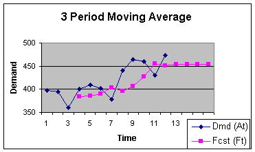
Figure 2.2.2 illustrates the lag that is present when using the moving average technique with a time series that exhibits a trend.

Figure 2.2.2




Five Period Moving Average Forecast
Here is "The Management Scientist" solution for using 5 periods to construct the moving average forecast.

Printout 2.2.2

FORECASTING WITH MOVING AVERAGES

********************************

THE MOVING AVERAGE USES 5 TIME PERIODS

TIME PERIOD TIME SERIES VALUE FORECAST FORECAST ERROR

=========== ================= ======== ==============

TIME PERIOD	TIME SERIES VALUE	FORECAST	FORECAST ERROR
1	398
2	395
3	361
4	400
5	410
6	402	392.80	9.20
7	378	393.60	-15.60
8	440	390.20	49.80
9	465	406.00	59.00
10	460	419.00	41.00
11	430	429.00	1.00
12	473	434.60	38.40

THE MEAN SQUARE ERROR 1,349.37

THE FORECAST FOR PERIOD 13 453.60


The RMSE for the Five-Period Moving Average forecast is 36.7, which is about 16% worse than the error of the three- period model. The reason for this is that there is a growth trend in this data. As we increase the number of periods in the computation of the moving average, the average begins to lag the growth trend by greater amounts. The same would be true if the historical data exhibited a downward trend. The moving average would lag the trend and provide forecasts that would be above the actual.

Pause and Reflect
The moving average forecasting method is simple to use and understand, and it works well with time series that do not have trend, seasonal or cyclical components. The technique requires little data, only enough past observations to match the number of time periods in in the moving average. Forecasts are usually limited to one period ahead. The technique does not work well with data that is not stationary - data that exhibits trend, seasonality, and/or cyclic patterns.

One-Period Moving Average Forecast or the "Naive Forecast"
A naive forecast would be one where the number of periods in the moving average is set equal to one. That is, the next forecast is equal to the last actual demand. Don't laugh! This technique might be useful in the case of rapid growth trend; the forecast would only lag the actual by one quarter or by one month, whatever the time period of interest. Of course, it would be much better to use a model that can make a trend projection if the trend represents a real move from a prior stationary pattern - we will get to that a bit later. Here is The Management Scientist result for the One-Period Moving Average Forecast.

Printout 2.2.3

FORECASTING WITH MOVING AVERAGES

********************************

THE MOVING AVERAGE USES 1 TIME PERIODS

TIME PERIOD TIME SERIES VALUE FORECAST FORECAST ERROR

=========== ================= ======== ==============

TIME PERIOD	TIME SERIES VALUE	FORECAST	FORECAST ERROR
1	398
2	395	398.00	-3.00
3	361	395.00	-34.00
4	400	361.00	39.00
5	410	400.00	10.00
6	402	410.00	-8.00
7	378	402.00	-24.00
8	440	378.00	62.00
9	465	440.00	25.00
10	460	465.00	-5.00
11	430	460.00	-30.00
12	473	430.00	43.00

THE MEAN SQUARE ERROR 969.91

THE FORECAST FOR PERIOD 13 473.00


This printout reflects a slightly lower RMSE than the three period moving average. That concludes our introduction to smoothing techniques by examining the class of smoothing methods called moving averages. The last smoothing method we will examine is called exponential smoothing, which is a form of a weighted moving average method.


Exponential Smoothing
This smoothing model became very popular with the production and inventory control community in the early days of computer applications because it did not need much memory, and allowed the manager some judgment input capability. That is, exponential smoothing includes a smoothing parameter that is used to weight either past forecasts (places emphasis on the average component) or the last observation (places emphasis on a rapid growth or decline trend component).

The exponential smoothing model is:

F_t+1 = a Y_t + (1 - a) F_t

where

F_t+1 = forecast of the time series for period t + 1
Y_t = actual value of the time series in period t
F_t = forecast of the time series for period t
a = smoothing constant or parameter (0 < a < 1)

The smoothing constant or parameter, a, is shown as the Greek symbol alpha in the text - I am limited to alpha characters. In any case, if the smoothing constant is set at 1, the formula becomes the naive model we already studied:

F_t+1 = Y_t

If the smoothing constant is set at 0, the formula becomes a weighted average model which gives most weight to the most recent forecast, with diminishing weight the farther back in the time series.

F_t+1 = F_t

Setting a can be done by trial and error, perhaps trying 0.1, 0.5 and 0.9, recording the RMSE for each run, then choosing the value of a that gives forecasts with the lowest RMSE. Some guidelines are, set a relatively high when there is a trend and you want the model to be responsive; set a relatively low when there is just the irregular component so the model will not be responding to random movements.

Let's do some exponential smoothing forecasts with a set at 0.6, relatively high.
To get the model started, we begin by making a forecast for Period 2 simply based on the actual demand for Period 1 (first shown in Table 2.2.1, but often repeated with each demonstration).

F₂ = Y₁ = 398

Then the first exponential smoothing forecast is actually made for Period 3, using information from Period 2. Thus t = 2, t+1 = 3, and F_t+1 = F₂₊₁ = F₃. For this forecast, we need the actual demand for Period 2 (Y_t = Y₂ = 395), the forecast for Period 2 (F₂ = 398. The result is:

F₃ = a Y₂+ (1 - a) F₂ = 0.6 (395) + (1-0.6) (398) = 396.2

The next forecast is for Period 4:

F₄ = a Y₃+ (1 - a) F₃ = 0.6 (361) + (1-0.6) (396.2) = 375.08

This continues through the data until we get to the end of Period 12 and are ready to make our last forecast for Period 13. Note that all we have to maintain in historical data is the last forecast, the last actual demand and the value of the smoothing parameter - that is why the technique was so popular since it did not take much data. However, I do not subscribe to "throwing away" data files today - they should be archived for audit trail purposes. Anyway, the forecast for Period 13:

F₁₃ = a Y₁₂+ (1 - a) F₁₂ = 0.6 (473) + (1-0.6) (439.86) = 459.74

Thankfully today, we have software like The Management Scientist to do the computations. To use The Management Scientist, select the Forecasting Module and load the data as previously described in the Three Period Moving Average demonstration. Next, click Solution/Solve/Exponential Smoothing and enter 0.6 where it asks for the value of the smoothing constant . Printout 2.2.4 illustrates the computer output with a smoothing constant of 0.6.

Printout 2.2.4

FORECASTING WITH EXPONENTIAL SMOOTHING

**************************************

THE SMOOTHING CONSTANT IS 0.6

 TIME PERIOD TIME SERIES VALUE FORECAST FORECAST ERROR

=========== ================= ======== ==============

TIME PERIOD	TIME SERIES VALUE	FORECAST	FORECAST ERROR
1	398
2	395	398.00	-3.00
3	361	396.20	-35.20
4	400	375.08	24.29
5	410	390.03	19.97
6	402	402.01	-0.01
7	378	402.01	-24.01
8	440	387.60	52.40
9	465	419.04	45.96
10	460	446.62	13.38
11	430	454.65	-24.65
12	473	439.86	33.14

THE MEAN SQUARE ERROR 871.52

THE FORECAST FOR PERIOD 13 459.74


This model provides a single forecast since, like the moving average techniques, it does not have the capability to address the trend component. The Root Mean Square Error is 29.52, (square root of the mean square error), or slightly better than the best results of the moving average and naive techniques.

However, since the time series shows trend, we should be able to do much better with the trend projection model that is demonstrated next.

Pause and Reflect
The exponential smoothing technique is a simple technique that requires only five to ten historical observations to set the value of the smoothing parameter, then only the most recent actual observation and forecasting values. Forecasts are usually limited to one period ahead. The technique works best for time series that are stationary, that is, do not exhibit trend, seasonality and/or cyclic components. While historical data is generally used to "fit the model" - that is set the value of a, analysts may adjust that value in light of information reflecting changes to time series patterns.

2.3: Trend Projections

When a time series reflects a shift from a stationary pattern to real growth or decline in the time series variable of interest (e.g., product demand or student enrollment at the university), that time series is demonstrating the trend component. The trend projection method of time series forecasting is based on the simple linear regression model. However, we generally do not require the rigid assumptions of linear regression (normal distribution of the error component, constant variance of the error component, and so forth), only that the past linear trend pattern will continue into the future. Note that is the trend pattern reflects a curve, we would have to rely on the more sophisticated features of multiple regression.

The trend projection model is:

T_t = b₀ + b₁ t

where,

T_t = Trend value for variable of interest in Period t
b₀ = Intercept of the trend projection line
b₁ = Slope, or rate of change, for the trend projection line

While the text illustrates the computational formulas for the trend projection model, we will use The Management Scientist. To use The Management Scientist, select the Forecasting Module and load the data as previously described in the Three Period Moving Average demonstration. Next, click Solution/Solve/Trend Projection and enter 4 where it asks for "Number of Periods to Forecast." Note, this is the first method that we have covered that the software asks this question, as it is assumed that all of the smoothing methods covered in this course are limited to forecasting just one period ahead.


Printout 2.3.1 illustrates the trend projection printout from The Management Scientist.

Printout 2.3.1

FORECASTING WITH LINEAR TREND

*****************************

THE LINEAR TREND EQUATION:

T = 367.121 + 7.776 t

where T = trend value of the time series in period t

 TIME PERIOD TIME SERIES VALUE FORECAST FORECAST ERROR

=========== ================= ======== ==============

TIME PERIOD	TIME SERIES VALUE	FORECAST	FORECAST ERROR
1	398	374.90	23.10
2	395	382.67	12.33
3	361	390.45	-29.45
4	400	398.23	1.78
5	410	406.00	4.00
6	402	413.78	-11.78
7	378	421.55	-43.55
8	440	429.33	10.67
9	465	437.11	27.90
10	460	444.88	15.12
11	430	452.66	-22.66
12	473	460.43	12.57

THE MEAN SQUARE ERROR 449.96

THE FORECAST FOR PERIOD 13 468.21

THE FORECAST FOR PERIOD 14 475.99

THE FORECAST FOR PERIOD 15 483.76

THE FORECAST FOR PERIOD 16 491.54


Now we are getting somewhere with a forecast! Note the mean square error is down to 449.96, giving a root mean square error of 21.2. Compared to the three period moving average RMSE of 31.7, we have a 33% improvement in the accuracy of the forecast over the relevant period.

Now, if this were products such as automobiles, to achieve a customer service level of 97.5%, we would create a safety stock of 2 times the RMSE above the forecast. So, for Period 13, the forecast plus 2 times the RMSE is 468.21 + (2 * 21.2) or 511 cars. With the three period moving average method, the same customer service level inventory position would be: 454.3 + (2 * 31.7) or 518. The safety stocks are 2 times 21 (42 for the trend projection) compared to 2 times 31.7 (63 for the three period moving average). This is a difference of 21 cars which could represent significant inventory carrying cost that could be avoided with the better forecasting method.

Note that the software provides the trend equation, showing the intercept of 367.121 and the slope of 7.776. The slope is interpreted as in simple linear regression, demand goes up 7.776 per unit increase in time. This means that over the course of the time series, demand is increasing about 8 units a quarter. The intercept is only of interest in placing the trend projection line on a time series graph. I used the Chart Wizard in Excel to produce such a graph for the trend projection model:


Figure 2.3.1



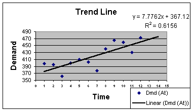
Note in this figure that demand falls below the trend projection line in Periods 3, 7 and 11. This is confirmed by looking at The Management Scientist computer Printout 2.3.1, where the errors are negative in the same periods. That is a pattern! Since our data is quarterly, we would suspect that there is a seasonal pattern that results in a valley in the time series in every third quarter.

To capture that pattern, we need the time series decomposition model that breaks down, analyzes and forecasts the seasonal as well as the trend components. We do that in the last section of this notes modules.

Pause and Reflect
The trend projection model is appropriate when the time series exhibits a linear trend component that is assumed to continue into the future. While rules of thumb suggest 20 observations to compute and test parameters of linear regression models, the simple trend projection model can be created with a minimum of 10 observations. The trend projection model is generally used to make multiple period forecasts for the short range, although some firms use it for the intermediate range as well.

2.4: Trend and Seasonal Components

The last time series forecasting method that we examine is very powerful in that it can be used to make forecasts with time series that exhibit trend and seasonal components. The method is most often referred to as Time Series Decomposition, since the technique involves breaking down and analyzing a time series to identify the seasonal component in what are called seasonal indexes. The seasonal indexes are used to "deseasonalize" the time series. The deseasonalized time series is then used to identify the trend projection line used to make a deseasonalized projection. Lastly, seasonal indexes are used to seasonalize the trend projection. Let's illustrate how this works. As usual, we will use The Management Scientist to do our work after the illustration.


The Seasonal Component
The seasonal component may be found by using the centered moving average approach as presented in the text, or by using the season average to grand average approach described here. The latter is a simpler technique to understand, and comes very close to the centered moving average approach for most time series.

The first step is to gather observations from the same quarter and find their average. I will repeat Table 2.2.1 as Table 2.4.1, so we can easily find the data:


Table 2.4.1

Time	Quarter	Actual Demand
1	1	398
2	2	395
3	3	361
4	4	400
5	1	410
6	2	402
7	3	378
8	4	440
9	1	465
10	2	460
11	3	430
12	4	473
13	1
14	2
15	3
16	4

To compute the average demand for Quarter 1, we gather all observations for Quarter 1 and find their average, then repeat for Quarters 2, 3 and 4:

Quarter 1 Average = (398 + 410 + 465) / 3 = 424.3
Quarter 2 Average = (395 + 402 + 460) / 3 = 419
Quarter 3 Average = (361 + 378 + 430) / 3 = 389.7
Quarter 4 Average = (400 + 440 + 473) / 3 = 437.7

The next step is to find the seasonal indexes for each quarter. This is done by dividing the quarterly average from above, by the grand average of all observations.

Grand Average = (398+395+361+400+410+402+378+

440+465+460+430+473) / 12 = 417.7

Seasonal Index, Quarter 1 = 424.3 / 417.7 = 1.016
Seasonal Index, Quarter 2 = 419 / 417.7 = 1.003
Seasonal Index, Quarter 3 = 389.7 / 417.7 = 0.933
Seasonal Index, Quarter 4 = 437.7/ 417.7 = 1.048

These indexes are interpreted as follows. The overall demand for Quarter 4 is 4.5 percent above the average demand, thus making Quarter 4 a "peak quarter." The overall demand for Quarter 3 is 6.7 percent below the average demand, thus making Quarter 3 an "off peak" quarter. This confirms our suspicion that demand is seasonal, and we have quantified the nature of the seasonality for planning purposes.

Please note The Management Scientist software Printout 2.4.1 provides indexes of 1.046, 1.009, 0.920, and 1.025. The peaks and off peaks are similar to the above computations, although the specific values are a bit different. The centered moving average approach used by the software requires more data for computations - at least 4 or 5 repeats of the seasons, we only have 3 repeats (12 quarters gives 3 years of data).

We will let the computer program do the next steps, but I will illustrate with a couple of examples. The next task is to "deseasonalize" the data. We do this by dividing each actual observation by the appropriate seasonal index. So for the first observation, where actual demand was 398, we note that it is a first quarter observation. The deseasonalized value for 398 is:

Deseasonalized Y₁ = 398 / 1.016 = 391.7

Actual demand would have been 391.7 if there was no seasonal effects. Let's do four more:

Deseasonalized Y₂ = 395 / 1.003 = 393.8
Deseasonalized Y₃ = 361 / 0.933 = 386.9
Deseasonalized Y₄= 400 / 1.048 = 381.7
Deseasonalized Y₅ = 410 / 1.016 = 403.6

I am sure you have seen "deseasonalized" numbers in articles in the Wall Street Journal or other popular business press and journals. This is how those are computed.

The next step is to find the trend line projection based on the deseasonalized observations. This trend line is a bit more accurate than the trend line projection based on the actual observations since than line contains seasonal variation. The Management Scientist gives the following trend line for this data:

T_t = 363 + 8.4 t

This trend line a close to the line we computed in Section 2.3, when the line was fit to the actual, rather than the seasonal data: T_t = 367 + 7.8 t.

Once we have the trend line, making a forecast is easy. Let's say we want to make a forecast for time period 2.

F₂ = T₂ * S₂ = [363 + 8.4 ( 2 ) ] * 1.009 = 379.8 * 1.009 = 383.2

Of course, The Management Scientist does all this for us. To use The Management Scientist, select the Forecasting Module and load the data as previously described in the Three Period Moving Average demonstration. Next, click Solution/Solve/Trend and Seasonal, then enter 4 where it asks for number of seasons, and 4 where it asks for number of periods to forecast. - click OK to get the solution.

Note that number of seasons is 4 for quarterly data, 12 for monthly data, and so forth. Here is the printout.


Printout 2.4.1

FORECASTING WITH TREND AND SEASONAL COMPONENTS

**********************************************

 SEASON SEASONAL INDEX

------ --------------

1 1.046

2 1.009

3 0.920

4 1.025

TIME PERIOD TIME SERIES VALUE FORECAST FORECAST ERROR

=========== ================= ======== ==============

TIME PERIOD	TIME SERIES VALUE	FORECAST	FORECAST ERROR
1	398	388.49	9.51
2	395	383.25	11.75
3	361	357..42	3.58
4	400	406.60	-6.60
5	410	423.81	-13.81
6	402	417.32	-15.32
7	378	388.49	-10.49
8	440	441.20	-1.20
9	465	459.12	5.88
10	460	451.38	8.62
11	430	419.57	10.43
12	473	475.80	-2.80

 

THE MEAN SQUARE ERROR 87.25

THE FORECAST FOR PERIOD 13 494.43

THE FORECAST FOR PERIOD 14 485.44

THE FORECAST FOR PERIOD 15 450.64

THE FORECAST FOR PERIOD 16 510.40


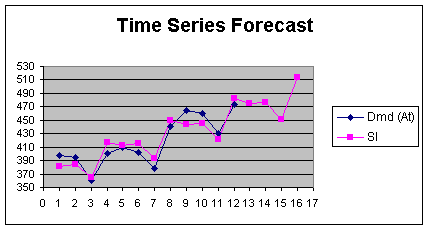
The Mean Square Error of 87.25, gives a root mean square error of 9.3, a spectacular improvement over the other techniques. A sketch of the actual and forecast data shows how well the trend and seasonal model can do at responding to the trend and the seasonal turn points. Note how the four period out forecast continues the response to both components.

Figure 2.4.1

Pause and Reflect
The trend and seasonal components method is appropriate when the time series exhibits a linear trend and seasonality. This model, compared to the others, does require significantly more historical data. It is suggested that you should have enough data to see at least four or five repetitions of the seasonal peaks and off peaks (with quarterly data, there should be 16 to 20 observations; with monthly data, there should be 48 to 60 observations).

Well, that's it to the introduction to times series forecasting material. Texts devoted entirely to this subject go into much more detail, of course. For example, there are exponential smoothing models that incorporate trend; and time series decomposition models that incorporate the cyclic component. A good reference for these is Wilson and Keating, Business Forecasting, 2nd ed., Irwin (1994).

Two parting thoughts. In each of the "Pause and Reflect" paragraphs, I gave suggestions for number of observations in the historical data base. There is always some judgment required here. While we need a lot of data to fit the trend and trend and seasonal models, "a lot of data" may mean going far into the past. When we go far into the past, the patterns in the data may be different, and the time series forecasting models assume that any patterns in the past will continue into the future (not the values of the past observations, but the patterns such as slope and seasonal indexes). When worded on forecasts for airport traffic, we would love to go back 10 years, but tourist and permanent resident business travel is different today than 10 years ago so we must balance the need for a lot of data with the assumption of forecasting.

The second thought is to always remember to measure the accuracy of your models. We ended with a model that had a root mean square error that was a 75% improvement over the 5-period moving average. I know one company that always used a 5-period moving average for their sales forecasts - scary, isn't it?

You should be ready to tackle the assignment for Module 2, "Forecasting Lost Sales," in the text, pp. 210-212. The case answers via e-mail and The Management Scientist computer output files are due February 10, 2001. If you want "free" review of your draft responses/output, please forward as a draft by Tuesday, February 6, 2001.