Module 3.2: Curvature, Dummy Variables and Interaction

Module 3.2 Notes
"Curvature, Dummy Variables and Interaction"

Index to Module Three Notes

3.1: Introduction to Multiple Regression

3.2: Curvature, Dummy Variables and Interaction

Multiple regression gives us the capability to add more than just numerical (also called quantitative) independent variables. In these notes, we will examine the curvilinear relationship between the dependent and independent variable, dummy variables and interaction. To illustrate all three concepts, I want to introduce a new example (I think I just heard some applause).

This example is near and dear to me: it involves a study of faculty pay. Here is the data. Years of experience (Years) is the independent variable hypothesized to predict Salary, the dependent variable.

Worksheet 3.2.1.

Years	Salary
13	72000
13	68000
10	66000
10	64000
14	64000
8	62000
15	61000
11	60000
9	60000
15	59000
5	59000
12	59000
11	58000
6	57000
7	56000
12	55000
6	55000
9	52000
14	51000
7	50000
3	45000
3	44000
4	44000
4	42000
8	41000
5	34000
2	34000
1	30000
2	25000
1	22000

Review of Linear Relationships

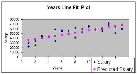
Suppose I wish to test a simple linear relationship between Salary and Years. The scatter diagram with the predicted linear regression equation is shown in the Worksheet 3.2.2 Line Fit Plot.

Worksheet 3.2.2

To determine if the linear regression has utility, I created the regression summary shown in Worksheet 3.2.3 by using the Regression Add-In Data Analysis Tool.

Worksheet 3.2.3

SUMMARY OUTPUT

Regression Statistics
Multiple R	0.786315511
R Square	0.618292083
Adjusted R Square	0.604659658
Standard Error	8132.062603
Observations	30

ANOVA
	df	SS	MS	F	Significance F
Regression	1	2999314286	2999314286	45.35451733	2.59764E-07
Residual	28	1851652381	66130442.18
Total	29	4850966667

	Coefficients	Standard Error	t Stat	P-value	Lower 95%	Upper 95%
Intercept	33119.04762	3124.438012	10.6000015	2.61857E-11	26718.91929	39519.17594
Years	2314.285714	343.6423654	6.734576255	2.59764E-07	1610.365448	3018.20598

The Summary Output provides the linear regression equation intercept and slope:

Eq. 3.2.1: Salary = 33119 + 2314 (Years)

The intercept of $33,119 is the salary a faculty member would make with no experience (a new hire). However, I can't be sure of this since we did not have any years of experience equal to zero in the sample. The slope of $2,314 indicates that salary increases $2,314 for every year of experience.

Recall that our test for practical utility looks at R Square (or R²) and the Standard Error of the Model. The R Square is 0.62, meaning that Years explain 62% of the sample variation in Salary in this linear model. That is above the benchmark of 0.50. The correlation coefficient of 0.79 confirms the moderate strength. The standard error of $8,132 means that we would expect 95% of the actual salaries to be within $16,264 (two times the standard error) of predicted salaries. This seems a bit high for practical utility. We can hold that thought and take a look at the assumptions.

To test for statistical utility, we set up the null and alternative hypotheses:

H₀: B₁ = 0 (linear regression model is not statistically useful)
H_a: B₁ =/= 0 (linear regression model is statistically useful)

Since the p-value (2.598E-07) for the t-Stat is less than alpha of 0.05, we reject the null hypothesis and conclude that the model has statistical utility.

To check the normality assumption for the errors or residuals, I checked for outliers and there were none in the standardized residual printout (I did not include these in Worksheet 3.2.2). Next, I produced the residual plot to check for the assumptions of constant error variance and independent errors. This is reproduced in Worksheet 3.2.4.

Worksheet 3.2.4

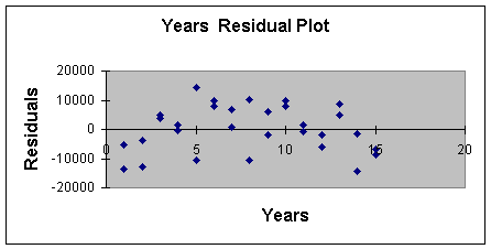
Note that for low values of Years, the observations are below the zero error line, then mostly above the line (up to 10), and then start to go back below the line of zero error. This pattern indicates that the last two assumptions are not satisfied and we may get a better model for prediction if we added curvature.

Curvilinear Relationships

The hypothesized regression model with curvature is as follows:

Eq. 3.2.2: E(Y) = B₀ + B₁X + B₂X²; for this example:

Salary = B₀ + B₁(Years) + B₂(Years)²

This equation is called the quadratic equation.

To add curvature, we simply create a new variable by squaring the quantitative independent variable, as shown in Worksheet 3.2.5. On the Excel Spreadsheet, I inserted a new column between Years and Salary. Then in Cell B2, I entered the formula =A2*A2 (you could also use the formula =A2^2) to get the squared term. I copied this down in Column B to square all of the years.

Worksheet 3.2.5

Years	Years^2	Salary
13	169	72000
13	169	68000
10	100	66000
10	100	64000
14	196	64000
8	64	62000
15	225	61000
11	121	60000
9	81	60000
15	225	59000
5	25	59000
12	144	59000
11	121	58000
6	36	57000
7	49	56000
12	144	55000
6	36	55000
9	81	52000
14	196	51000
7	49	50000
3	9	45000
3	9	44000
4	16	44000
4	16	42000
8	64	41000
5	25	34000
2	4	34000
1	1	30000
2	4	25000
1	1	22000

Next, I got the Regression Summary by running the Regression Data Analysis Add-In under the Tools icon on the Standard Toolbar, just as we have done many times by now. Remember to increase your selection for the X Range by including both columns of Years and Years^2 (for Years Squared). The Regression Summary Results are shown in Worksheet 3.2.6.

Worksheet 3.2.6


SUMMARY OUTPUT

Regression Statistics
Multiple R	0.860591031
R Square	0.740616923
Adjusted R Square	0.721403361
Standard Error	6826.578401
Observations	30

ANOVA
	df	SS	MS	F	Significance F
Regression	2	3592708005	1.8E+09	38.54657	1.22521E-08
Residual	27	1258258662	46602173
Total	29	4850966667

	Coefficients	Standard Error	t Stat	P-value	Lower 95%	Upper 95%
Intercept	20961.53846	4299.678538	4.875141	4.26E-05	12139.33274	29783.74
Years	6605.171299	1236.600525	5.341395	1.22E-05	4067.878304	9142.464
Years^2	-268.1803491	75.15511808	-3.56836	0.00137	-422.3858105	-113.975

The coefficients for the multiple regression equation with curvature are provided in the rows labeled Intercept, Years and Years^2. The equation based on the sample is:

Eq. 3.2.3: Salary = 20961.5 + 6605.2 (Years) - 268.18 (Years)²

The intercept may be interpreted similar to simple linear regression. Salary is $20,961.5 for faculty with no years of service in this curvilinear model. Again, this is not a practical interpretation since we had no faculty with zero years of service in the data base.

The coefficient for Years Squared (-268.18) is a negative number meaning that the curvature is negative. The interpretation of the negative curvature is simply that as Years (X) increase, Salary (Y) increases at a decreasing rate. Note that a positive coefficient on the curvature variable would mean that as X increases, Y increases at an increasing rate. The coefficient for Years, 6605.2, has no managerial interpretation. It simply locates the curve on the XY axis.

Let's look at the line fit plot to see what negative curvature looks like (Worksheet 3.2.7). As you recall, the line fit plot is part of the automatic output of the Regression Add-In provided you check the Line Fit Plot Residual Output Option.

Worksheet 3.2.7

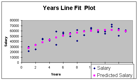
There is actually a name for the negative curve shape - it's called concave. Positive curve shape looks like a cross section of a bowl - it's called convex.

This model has better practical utility than the simple linear regression model. The Adjusted R Square climbed to 0.72, compared to 0.62 for the simple linear regression model. The Standard Error decreased from $8,132 to $$6,828. Still high, but it's an improvement.

To test for statistical utility, we can first do a model test.

H₀: B₁ = B₂ = 0 (regression model is not statistically useful)
H_a: at lease one B =/= 0 (regression model is statistically useful)

Since the p-value (1.22521E-08) for the F is less than alpha of 0.01, we reject the null hypothesis and conclude that the model is statistically useful. Now, for our test on curvature. The hypotheses are:

H₀: B₂ = 0 (curvature is not important or curvature is not present)
H_a: B₂ =/= 0 (curvature is important)

Since the p-value for the t-stat for the Years^2 curvature term is less than alpha of 0.01, we reject the null hypothesis and conclude that curvature is important. Since Years^2is important, we do not need to do a separate test on Years since the Years variable is required to produce Years^2.

To check the normality assumption for the errors or residuals, I checked for outliers and there were none in the standardized residual printout (I did not include these in Worksheet 3.2.6 ). Next, I produced the residual plot to check for the assumptions of constant error variance and independent errors. This is reproduced in Worksheet 3.2.8.

Worksheet 3.2.8.

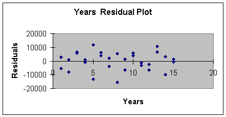
Although the magnitude of the variation starts small, gets larger, gets small again and so forth, adding curvature did remove the negative/positive/negative pattern. We will see even more improvement when we add the categorical or dummy variable.

The last step in the regression procedure is to make the prediction. Suppose we want to predict the salary for a professor with 10 years experience. The point estimate is:

Eq. 3.2.4: Salary = 20961.5 +6605.2 (10) -268.18 (10)² = $60,196

Adding the prediction interval gives us the following. We are 95% confident that a faculty member with 10 years experience will make a salary between $46,542 and $73,850, as shown in Eq. 3.2.5.

Eq. 3.2.5: Salary = $60,196 +/- (2 * Standard Error of Model)

Salary = $60,196 +/- (2 * $6,827)
Salary = $60,196 +/- $13,654

Next we will examine categorical or dummy variables.

Dummy Variables

Multiple regression gives us the capability to incorporate a very useful technique to stratify the data in our attempt to build more reliable and accurate prediction models. We stratify data by using dummy variables (also called categorical or qualitative variables).

Recall that the Standard Error of the Estimate of $6,827 for the curvilinear model is fairly high, even though it is much better than the Standard Error of the linear model. One reason that the error may be so high is that I am including both male and female faculty member in the database. If there is salary discrimination, combining both males and females would lead to high error. One solution is to run two separate models - one for females and one for males. Another option is to stratify or categorize males and females in one regression model. The benefit of stratification in one regression model is that we picture any differences in the line fit plots, and we can test for interaction which I cover last in this note set.

The way we stratify data is to categorize it by using a dummy variable. In this case, let's let X represent a variable called gender. It's values are:

X = 1 if the faculty member is male
X = 0 if the faculty member is female

Which gender gets the 1 and which gets the 0 is arbitrary, but only use 1 and 0 for the two categories (for example, do not use 2 and 1). Note that by using 0, the intercept will now have an interpretation. Worksheet 3.2.9 illustrates the data for a regression model with one dependent variable, Salary, and one independent variable, gender.

Worksheet 3.2.9

Gender	Salary
1	72000
0	68000
1	66000
0	64000
1	64000
1	62000
1	61000
0	60000
1	60000
0	59000
1	59000
1	59000
1	58000
0	57000
1	56000
0	55000
1	55000
0	52000
0	51000
0	50000
1	45000
0	44000
1	44000
0	42000
0	41000
0	34000
1	34000
1	30000
0	25000
0	22000

The first faculty member is a male making $72,000 (must be in the College of Medicine or Engineering), the second faculty member is a female, etc.

Worksheet 3.2.10 provides the regression Summary Output.

Worksheet 3.2.10

SUMMARY OUTPUT

Regression Statistics
Multiple R	0.264756482
R Square	0.070095995
Adjusted R Square	0.036885137
Standard Error	12692.70507
Observations	30

ANOVA
	df	SS	MS	F	Significance F
Regression	1	340033333.3	340033333.3	2.110634902	0.157394431
Residual	28	4510933333	161104761.9
Total	29	4850966667

	Coefficients	Standard Error	t Stat	P-value	Lower 95%	Upper 95%
Intercept	48266.66667	3277.242356	14.72782951	1.03073E-14	41553.53248	54979.80085
Gender	6733.333333	4634.720587	1.45280243	0.157394431	-2760.472079	16227.13875

The regression Summary Output provides the following regression equation:

Eq. 3.2.6: E(y) = b₀ + b₁x ; for this sample:

Salary = $48,267 + $6,733(Gender)

Recall that males were given the category 1 and females 0. So we can now make our point estimates of average male and female salaries:

Eq. 3.2.7: Salary = $48,267 + ($6,733 * 1) or $55,000 for males;

Salary = $48,267 + ($6,733 * 0) or $48,267 for females

The regression parameters take on a different interpretation for dummy variables. The "intercept" is the average salary made by females, and the "slope" is the difference between the average salaries made by males and females. Another difference with dummy variables is the line fit plot, since X only takes on values of 0 and 1. The line fit plot will show the cluster of female and male faculty actual observations at X = 0 and X = 1, and the prediction (average value for Y when X = 1, and average value for Y when X = 0) as points. Worksheet 3.2.11 illustrates the line fit plot.

Worksheet 3.2.11

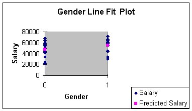
Generally, we use a dummy variable as a stratification variable along with one or more other independent variables. Indeed, you can see from the regression summary output that the regression model with just gender and salary does not have statistical or practical utility. We will combine the dummy variable with the experience independent variable in the next section to see if our results improve. I simply used the dummy variable by itself to introduce the concept.

Dummy variables are used to categorize data in models where there are attributes such as in season/out of season, large/small, and defective/not defective. You will be asked to incorporate a dummy variable in Assignment 3.

If the characteristic being modeled has more than two levels, we need to use more than one dummy variable. For example, what if you wanted to model Fall, Winter, Spring, Summer. Then, X₁ could represent Fall and if the observation is a Fall observation, it gets the value 1 in data entry, 0 otherwise; X₂ is used for Winter; and X₃ is used for Spring. There would be no dummy variable for Summer. Do you know why? Did I hear, "the intercept becomes Summer"? That's right!

For Assignment 3, we will be adding just one dummy variable, so keep to two levels (male/female, in season/out of season, large/small, etc.) .

The next modeling concept is interaction.

Interaction

When there are two independent variables, the relationship between Y and X₁ may depend on X₂: that dependency is called interaction. When the relationship between Y and X₁ does not depend on X₂ we say there is no interaction. I am going to illustrate the "no interaction" case first, since I can use the data in the faculty salary example. I will introduce a new data set to demonstrate "interaction" after that.

The hypothesized population equation to model interaction is:

Eq. 3.2.8: E(Y) = B₀ + B₁X₁ + B₂X₂ + B₃X₁X₂;

The cross-product term, X₁X₂, is the interaction term, so B₃ in Equation 3.2.8 is the slope of interest for testing interaction.

To model interaction with sample data, we multiple the two independent variables to make a new variable. Worksheet 3.2.12 illustrates multiplying the contents of the cells in Column A (Years) with the cells in Column B (Gender) to make a new variable, Yrs*Gndr.

Worksheet 3.2.12

Years	Gender	Yrs*Gndr	Salary
13	1	13	72000
13	0	0	68000
10	1	10	66000
10	0	0	64000
14	1	14	64000
8	1	8	62000
15	1	15	61000
11	0	0	60000
9	1	9	60000
15	0	0	59000
5	1	5	59000
12	1	12	59000
11	1	11	58000
6	0	0	57000
7	1	7	56000
12	0	0	55000
6	1	6	55000
9	0	0	52000
14	0	0	51000
7	0	0	50000
3	1	3	45000
3	0	0	44000
4	1	4	44000
4	0	0	42000
8	0	0	41000
5	0	0	34000
2	1	2	34000
1	1	1	30000
2	0	0	25000
1	0	0	22000

Worksheet 3.2.14 provides the regression Summary Output.

Worksheet 3.2.14

SUMMARY OUTPUT

Regression Statistics
Multiple R	0.830657322
R Square	0.689991587
Adjusted R Square	0.654221386
Standard Error	7605.262541
Observations	30

ANOVA
	df	SS	MS	F	Significance F
Regression	3	3347126190	1115708730	19.28956392	8.62451E-07
Residual	26	1503840476	57840018.32
Total	29	4850966667

	Coefficients	Standard Error	t Stat	P-value	Lower 95%	Upper 95%
Intercept	28809.52381	4132.381497	6.971651536	2.10919E-07	20315.28642	37303.76119
Years	2432.142857	454.5013685	5.351233298	1.33311E-05	1497.901302	3366.384412
Gender	8619.047619	5844.069958	1.474836489	0.152263821	-3393.618092	20631.71333
Yrs*Gndr	-235.7142857	642.7619995	-0.366720942	0.716794859	-1556.931363	1085.502792

The coefficients for the multiple regression model with interaction are provided in the rows labeled Intercept, Years, Gender and Yrs*Gndr. The equation based on this sample is:

Eq. 3.2.9: E(y) = b₀ + b₁x₁ + b₂x₂ + b₃x₃ + b₄x₁x₂; here

Salary = 28809.5 + 2432.1 (Years) +
8619 (Gender) - 235.7 (Yrs*Gndr)

To determine if interaction is important, we can proceed directly to the hypothesis test for interaction:

H₀: B₃ = 0 (interaction is not important)
H_a: B₃ =/= 0 (interaction is important)

Since the p-value (0.717) for the t-stat for the Yrs*Gndr term is greater than 0.01, we do not reject the null hypothesis and conclude interaction is not important. The analyst should then remove the interaction column of data and rerun the regression model without interaction to see if either years or gender or both are important in predicting salary. Worksheet 3.2.15 illustrates what "no interaction" looks like:

Worksheet 3.2.15

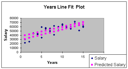
This line fit plot illustrates the relationship between Salary and Years. But note that there are two regression lines. The two regression lines represent the stratification of the data - one line for males and one for females. Can you guess which is the top line? Right - the male regression line is the top line. We learned that when we examined the gender variable in the previous section: males make more than females. There was, in fact, salary discrimination at the university where this data sample came from.

But because the two regression lines have approximately the same slope, we can predict the increase in salary for males or females based on time alone. I realize that males make more than females - but it is a fixed amount because the slopes are parallel. Thus, the formal definition of "no interaction" is, for this problem: the relationship between Salary and Years does not depend on gender. Recall that statistical relationships between variables in regression is measured through the slope. The slope on years is $2,432 for both males and females since the Years*Gender term goes away (the interaction slope is equal to zero).

IF there was interaction, then the slopes would be different for males and females. For an hypothetical example, what if the Equation 3.2.9 came out as follows:

Eq. 3.2.10: Salary = 28809.5 + 2432.1 (Years) + 8619 (Gender) +

1000 (Yrs*Gndr)

Now note what happens when we substitute 1 (for males) in the gender term:

Eq. 3.2.11: Male Salary = 28809.5 + 2432.1 (Years) + 8619 (1) +

1000 (1 * Years) = 37428.5 + 3432.1 (Years)

...and then 0 (for females) in the gender term

Eq. 3.2.12: Female Salary = 28809.5 + 2432.1 (Years) + 8619 (0)

+1000 (0 * Years) = 28809.5+ 2432.1 (Years)

In my hypothetical example, the slope for the male regression line is 3432.1; meaning that male salaries increase $3,432 per year. The slope for the female regression line is $2,432.1; meaning that female salaries increase only $2,432.1 per year. Since the slopes are different, we cannot predict the change in salary without knowing the gender. Thus, we would say there is interaction: the relationship between salary and years depends on whether the faculty member is male or female.

The above illustration of interaction was hypothetical. There really was no interaction but there really was discrimination - males made more on average than females, but that amount was constant for all levels of experience (no interaction). If the amount was not constant, there would have been interaction).

Let's examine an actual model of interaction so you can an actual picture and the equations for interaction. This example was an experiment done by an over-the-counter drug manufacturer interested in testing a new drug designed to be effective in curing an illness most commonly found in older patients. The dependent variable is Effect, which stands for the effectiveness of recovery from a certain illness. It is measured on a scale of 0 to 100 (100 is more effective). The quantitative independent variable is age, and the qualitative independent variable is whether or not the new drug was present (drug = 0) or absent (subjects took the old drug) (drug = 1) in the experiment. Note that half of the subjects were given the new drug, and half were given the old drug (they were not told which one to avoid bias in the experiment. This would then be called a blind experiment since the subjects did not know which drug they were taking. An experiment is called a double blind experiment if the drug administrator does not know which drug is being administered, as well. Worksheet 3.2.16 shows the data entry.

Worksheet 3.2.16

Age	Drug	Age*Drug	Effect
21	1	21	56
19	0	0	28
28	1	28	55
23	0	0	25
67	0	0	71
33	1	33	63
33	1	33	52
56	0	0	62
45	0	0	50
38	1	38	58
37	0	0	46
27	0	0	34
43	1	43	65
47	0	0	59
48	1	48	64
53	1	53	61
29	0	0	36
53	1	53	69
58	1	58	73
63	1	63	62
59	0	0	71
51	0	0	62
67	1	67	70
63	0	0	71

Worksheet 3.2.17 provides the regression summary.

Worksheet 3.2.17

SUMMARY OUTPUT

Regression Statistics
Multiple R	0.96551637
R Square	0.932221861
Adjusted R Square	0.92205514
Standard Error	3.87724774
Observations	24

ANOVA
	df	SS	MS	F	Significance F
Regression	3	4135.297333	1378.432444	91.69346477	7.33335E-12
Residual	20	300.6610008	15.03305004
Total	23	4435.958333

	Coefficients	Standard Error	t Stat	P-value	Lower 95%	Upper 95%
Intercept	6.211381194	3.308965648	1.877136802	0.075164685	-0.690996989	13.11375938
Age	1.033390871	0.071447502	14.46363902	4.70078E-12	0.884354064	1.182427679
Drug	41.30421013	5.022786373	8.223365889	7.5975E-08	30.82686622	51.78155404
Age*Drug	-0.702883614	0.10763568	-6.530210205	2.30245E-06	-0.927407604	-0.478359625

The Intercept, Age, Drug and Age*Drug regression coefficients provide the equation from this sample:

Eq. 3.2.13: Effect = 6.2+ 1.03 (Age)+ 41.3 (Drug) - 0.7 (Age*Drug)

Let's look at the equation for subjects who got the old drug (did not get the new drug) (drug = 1):

Eq. 3.2.14: Effect = 6.2 + 1.03 (Age) + 41.3 (1) - 0.7 (Age*1)

Effect = 47.5 + 0.33 (Age)

Now, look at the equation for subjects who got the new drug (drug = 0):

Eq. 3.2.15: Effect = 6.2 + 1.03 (Age) + 41.3 (0) - 0.7 (Age*0)

Effect = 6.2 + 1.03 (Age)

Subjects who got the new drug would enjoy a nearly a 1 unit increase in drug healing effectiveness for each year of age. On the other hand, subjects who got the old drug only enjoy a .33 unit increase in effectiveness for each year of age. The drug manufacturer would be excited about this finding - the new drug is more effective as one ages. Statistically, we say there is interaction. The relationship between effectiveness and age depends on whether or not the subject is taking the drug. The slopes of the regression equation change when there is interaction.

Worksheet 3.2.18

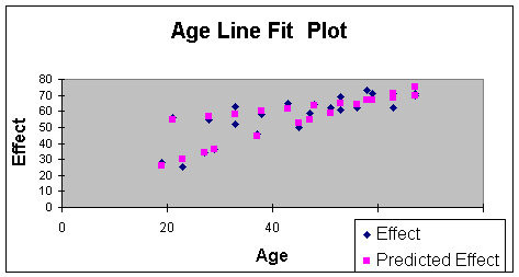
In the Worksheet 3.2.18 Line Fit Plot, note the steeper sloping line that begins with the observation of a subject aged 20, with an effectiveness score of just below 30. This is the line of Equation 3.2.15 - the one with the steeper slope that shows more effectiveness with age than line of Equation 3.2.14. The drug manufacturer can then tell that for subjects over 60, there should be more effectiveness in healing with the new drug as patients age. I will use this example again in Module Notes 3.2.3 when we discuss model building. I will go over statistical and practical utility, testing assumptions and prediction with this model at that time. This illustration was simply used to show a picture of interaction.

That's it! We now talked about the separate components of multiple regression. Adding a quantitative independent variable, adding a qualitative (dummy) independent variables, adding a curvature component, and adding an interaction component. There can be more complications - such as adding several more quantitative variables and studying three-way interactions - but you have the basic building blocks of multiple regression involving a quantitative dependent variable. Note that because of the principle of parsimony, I would suggest caution before building a model that has so many terms it is impossible to interpret.

There are model extensions for qualitative dependent variables but they go beyond the scope of this course.
All that remains for our study of multiple regression is a system for knowing how to put the separate components together in a single model. That is the subject of Module Notes 3.3.

References:

Anderson, D., Sweeney, D., & Williams, T. (2007). Contemporary Business Statistics with Microsoft Excel. Cincinnati, OH: 3^rd Edition, South-Western, Chapter 13 (Section 13.7).

D. Groebner, P. Shannon, P. Fry & K. Smith. Business Statistics: A Decision Making Approach, Seventh Edition, Prentice Hall, Chapter 15.

Ken Black. Business Statistics for Contemporary Decision Making. Fourth Edition, Wiley. Chapter 13, 14 & 15 (Advanced chapter: 16).

Levine, D., Berenson, M. & Stephan, D. (1999). Statistics for Managers Using Microsoft Excel (2nd. ed.). Upper Saddle River, NJ: Prentice-Hall. Chapter 14 -- Multiple Regression Models.

Mason, R., Lind, D. & Marchal, W. (1999). Statistical Techniques in Business and Economics (10th. ed.). Boston: Irwin McGraw Hill. Chapter 13 -- Multiple Regression and Correlation Analysis

| Return to Module Overview | Return to top of page |