|
Index to Module Three Notes
|
To recap, multiple regression
allows us to study the relationship between a dependent variable and multiple
independent variables. The independent variables can be numerical
(quantitative) or dummy (qualitative or categorical) variables. They can also
be functions of independent variables, such as the curvature component and/or
the interaction component. So how do we know what component to put into the
multiple regression model?
You could always use trial and error - but that isn't good science. Formal techniques
include forward selection (start with a simple linear regression model and add
predictor variables as long as significant improvement is made); backward
selection (start with a large pool of predictor variables and successively
remove variables that do not significantly contribute to the prediction);
stepwise regression (like forward selection but variables once added are also
tested for removal after subsequent addition of more variables to determine if
better models result); and best subsets (create subsets or combinations of all
predictor variables and select the model with best statistical and practical
utility). The Handbook of Parametric and Non parametric Statistical
Procedures, by David Sheskin provides more details on the various methods.
The approach I would like you to use in Assignment 3 is a modification of the
backward selection method. We will hypothesis a full multiple regression model
with a quantitative independent variable, qualitative independent variable,
curvature and interaction. We will then start taking components away that do
not contribute to the statistical utility of the model. However, the way we
take components away will be by following a decision tree in order to give us
some structure.
In getting ready for Assignment 3, the first item is to enter your data into an
Excel Spreadsheet, and create the interaction term. I will demonstrate how to
do this with several examples later in these notes. Item 2 requires that you
build and test at least 2 of the hypothesized models shown in the next section,
starting with Model 1 (Item 3 of Assignment 3).
Hypothesized
Models
The decision tree will "walk us through" the selection of one of the
following seven models that best fits the sample of data for your Assignment 3.
The symbol QN stands for your quantitative X, QL represents the qualitative X,
and QN*QL represents interaction.
Model 1: E(Y) = B0 + B1 QN + B2 QL + B3QN*QL
Model 2: E(Y) = B0 + B1 QN + B2 QL
Model 3: E(Y) = B0 + B2QL
Model 4: E(Y) = B0 + B1 QN
A word description for each model is that the hypothesized regression model for predicting Y includes:
Model 1:
Quantitative and qualitative variables, and interaction
Model 2: Quantitative and qualitative variables
Model 3: A qualitative variable
Model 4: A quantitative variable
To determine which model is
best your sample data, we use the following decision tree.
Model
Building Decision Tree
Item 3 in Assignment
3 asks you to run the Model 1 Regression Model. Item 4 in Assignment 3 requires
that you first test to determine if interaction is important in that model and
then a decision tree with the actions you should follow depending on the
outcome of that and subsequent tests.
A. Build Model 1 and test interaction.
(1). If interaction is significant, stop. Model 1 is "best" model. Go to item 5.
(2). If interaction is not significant, build Model 2 and test QL.
a. If QL is significant, test QN.
1. If QN is significant, stop. Model 2 is "best" model. Go to Item 5.
2. If QN is not significant, stop.
Model 3 is "best model. Go to Item 5.
b. If QL is not significant, stop and select Model 4 as "best" model, even if the Model is not significant. Go to Item 5.
Although Item 5 is not part of the decision tree, it is part of the Assignment 3 requirement so I am repeating it here for ready reference (the decision tree appear in the Main Module 3 Web Page).
5. Rerun the data analysis regression tool for your "best" model, and include and be able to describe or interpret the following printouts:
· Residual plot :
· Normal probability plot (for all Models)
· Fitted Line Plot:
Example
One: Drug Effectiveness
Item 1: Enter Data
I am going to use as my first example, the study introduced at the end of
Module Notes 3.2: the new drug effectiveness study data.
This example concerned an experiment done by an over-the-counter drug
manufacturer interested in testing a new drug. This drug is designed to be
effective in curing an illness most commonly found in older patients. The
dependent variable is Effect, which stands for the effectiveness of recovery
from a certain illness. It is measured on a scale of 0 to 100 (100 is more
effective). The quantitative independent variable is age, and the qualitative
independent variable is whether or not the new drug was present in the
experiment (drug = 0) or absent (subjects took the old drug, drug = 1) in the
experiment. Note that half of the subjects were given the new drug, and half
were given the old drug (they were not told which one to avoid bias in the
experiment).
Worksheet 3.3.1 shows the data entry (Item 1, Assignment 1).
Worksheet 3.3.1
|
Age |
Drug |
Age*Drug |
Effect |
|
21 |
1 |
21 |
56 |
|
19 |
0 |
0 |
28 |
|
28 |
1 |
28 |
55 |
|
23 |
0 |
0 |
25 |
|
67 |
0 |
0 |
71 |
|
33 |
1 |
33 |
63 |
|
33 |
1 |
33 |
52 |
|
56 |
0 |
0 |
62 |
|
45 |
0 |
0 |
50 |
|
38 |
1 |
38 |
58 |
|
37 |
0 |
0 |
46 |
|
27 |
0 |
0 |
34 |
|
43 |
1 |
43 |
65 |
|
47 |
0 |
0 |
59 |
|
48 |
1 |
48 |
64 |
|
53 |
1 |
53 |
61 |
|
29 |
0 |
0 |
36 |
|
53 |
1 |
53 |
69 |
|
58 |
1 |
58 |
73 |
|
63 |
1 |
63 |
62 |
|
59 |
0 |
0 |
71 |
|
51 |
0 |
0 |
62 |
|
67 |
1 |
67 |
70 |
|
63 |
0 |
0 |
71 |
I entered the quantitative X1, Age, in the first column. The second
column is the qualitative X2, drug (0 = new drug was present, 1 = new
drug was absent). The third column includes the interaction component, which is
obtained by multiplying the respective cells in the Age Column times the cells
in the Drug Column. I titled this Age*Drug to represent the multiplication.
Finally, the last column contains the quantitative Y variable.
You are free to set up your data as you wish; the above format seems to be most
efficient of the various formats I tried. Your requirement is similar to the
example above: one quantitative X1, one qualitative X2,
and a quantitative Y. Interaction is constructed!!
Item 2: Build Model 1
Item 2, Assignment 3,
requires that you hypothesize and run a full model with the quantitative and
qualitative variables and the interaction term.
Worksheet 3.3.2 illustrates the regression summary from using the Regression
Data Analysis Add In.
Worksheet 3.3.2
|
SUMMARY OUTPUT |
||||||
|
Regression
Statistics |
||||||
|
Multiple R |
0.965516 |
|||||
|
R Square |
0.932222 |
|||||
|
Adjusted R Square |
0.922055 |
|||||
|
Standard Error |
3.877248 |
|||||
|
Observations |
24 |
|||||
|
ANOVA |
||||||
|
|
df |
SS |
MS |
F |
Significance
F |
|
|
Regression |
3 |
4135.297 |
1378.432 |
91.69346 |
7.33335E-12 |
|
|
Residual |
20 |
300.661 |
15.03305 |
|||
|
Total |
23 |
4435.958 |
|
|
|
|
|
|
Coefficients |
Standard
Error |
t
Stat |
P-value |
Lower
95% |
Upper
95% |
|
Intercept |
6.211381 |
3.308966 |
1.877137 |
0.075165 |
-0.691000176 |
13.11376256 |
|
Age |
1.033391 |
0.071448 |
14.46364 |
4.7E-12 |
0.884353995 |
1.182427747 |
|
Drug |
41.30421 |
5.022786 |
8.223366 |
7.6E-08 |
30.82686138 |
51.78155887 |
|
Age*Drug |
-0.70288 |
0.107636 |
-6.53021 |
2.3E-06 |
-0.927407707 |
-0.478359521 |
First Test: Interaction
Item
4, Assignment 3, requires that we test interaction. This is where the decision
tree begins. Since we have the full Model 1 constructed, we can easily test for
interaction by comparing Model 1 to Model 2. Model 2 is just like Model 1
except it doesn't have interaction.
The slope coefficient that we need to use to test interaction is B3.
The null and alternate hypotheses to test interaction are:
H0:
B3 = 0 (interaction is not important)
Ha: B3 =/= 0 (interaction is important)
Note: I do not recommend selecting any of
the output options at this point. The Regression Summary is all that we need
for the various component test procedures in the decision tree. Once we have
our best model, we can rerun it and produce all of the output options such as
residual, normal and line fit plots.
The hypothesized model associated with the null hypothesis at this point in the decision tree is Model 2, and the hypothesized model associated with the alternative hypothesis is Model 1.
Model 2 Associates with H0: Effect = B0 + B1 Age + B2 Drug
Model 1 Associates with H1: Effect = B0 + B1 Age + B2Drug + B3 Age*Drug
Since the p-value (2.3E-06) for the interaction term (Age*Drug) in Worksheet 3.3.2 is less than alpha of 0.01, reject the null hypothesis, and conclude that interaction is important. This means that Model 1 is the best predictor. Note in the decision tree action A (1), that if interaction is important at this point in the tree, we stop, Model 1 is our best model. You see, we do not need to test if the quantitative or if the qualitative variables are important, since if interaction is important, we need both the quantitative and qualitative variables to create it (the interaction).
Item 5: Assignment 3
Now that you have
your best model, rerun the regression and select all of the output options of
the regression add in dialog box (residual, normal, and line fit plots and
standardized residuals). You are now ready to interpret the regression
coefficients, test practical utility of your model, test statistical utility of
your model, evaluate the assumptions and make a prediction.
The Sample Regression Equation and Interpretation of Coefficients
Worksheet 3.3.2 provides the coefficients for the sample regression
equation:
Eq. 3.3.1: Effect = 6.2 + 1.03 Age + 41.3 Drug - 0.7Age*Drug
Since this is an interaction model, we have two interpretations for the slope and intercept. For the case where drug = 0 (new drug), the equation becomes:
Eq. 3.3.2: Effect = 6.2 + 1.03 Age
The intercept means that the
Effectiveness score would be 6.2 for a person of age equals zero. Since there
were no subjects at that age, the intercept would not have practical meaning.
The slope suggests that when age increases by one, the effectiveness score
increases by 1.03 (again, holding the qualitative variable constant at drug =
0).
For the case where drug = 1 (old drug), the equation becomes:
Eq. 3.3.3: Effect = 47.5 + 0.33 Age
The intercept now means that
Effectiveness score would be 47.5 for a person of age equals zero. Since there
were no subjects at that age, the intercept would not have practical meaning.
The slope suggests that when age increases by one, the effectiveness score
increases by 0.33 (again, holding the qualitative variable constant at drug =
1).
Practical Utility
The Adjusted R Square for this multiple regression model is shown as 0.92.
The interpretation is that age and drug type explain 92% of the variation in
effectiveness score. This is a high degree of variation explained. The Standard
Error of the Model is 3.877, meaning that 95% of the actual effectiveness
scores would be within +/- 2 * 3.877 = 7.75) of predicted effectiveness scores.
This appears to be a relatively low standard error. The model is judged to be
practically useful.
Statistical Utility
The following hypothesis test is used to determine model utility.
H0: B1 = B2 = B3 = 0 (regression model is not statistically useful)
Ha: At least one B =/= 0 (regression model is statistically useful)
Since the p-value (7.33E-12)
for the F statistic in the Regression Row of the ANOVA table of Worksheet 3.3.2
is less than alpha of 0.01, reject the null hypothesis and conclude that the
model is statistically useful.
Assumptions
I examined the standardized residuals and the normal probability plot and
found no outliers, indicating that the assumption that the error terms are
normally distributed around a mean of zero can be considered met. To determine
if we meet the assumptions that the error has constant variance and is
independent, we examine the residual plots. There will be two plots since there
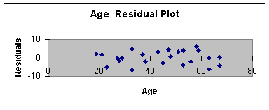
are two independent variables. Worksheet 3.3.4 provides the residual plot Age,
and Worksheet 3.3.5 provides the residual plot for Drug.
Worksheet 3.3.4
Worksheet 3.3.5
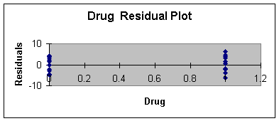
The plot of residual or errors against age shows fairly constant variance for
all values of Age. Likewise, the errors plotted against drug shows about the
same spread for drug = 0 and drug = 1.
Making a Prediction
To predict the effectiveness score for a new drug (drug = 0) administered a
63 year old, we first obtain the point estimate:
Eq. 3.3.4: Effect = 6.2 + 1.03Age + 41.3 Drug - 0.7 Age*Drug;
Effect
= 6.2 + 1.03 (63) + 41.3 (0) -0.7 (63*0);
Effect = 6.2 + 64.9 = 71.1
Next, incorporate two times the standard error to get the 95% prediction interval:
Eq. 3.3.5: Effect = 71.1 +/- (2 * 3.877) = 71.1 +/- 7.75
We are 95% confident that a
person 63 years of age, using the new drug, will have an effectiveness score
between 63.35 and 78.85.
Example
Two: Salary Study
Item 1: Enter Data
The second model building example concerns the Salary Study that was
introduced in Module Notes 3.2 to illustrate the concepts of dummy variable and
interaction. I will use that example here to demonstrate how to determine the
"best" model - that is, what combination of the independent variables
(quantitative variable, qualitative variable, and interaction) would best
predict faculty salary. For this example
we'll use a level of significance alpha equal to 0.05.
The data that had to be collected includes faculty salary (dependent variable,
Y), years of experience (quantitative independent variable, X1), and
gender (qualitative independent variable, X2). The data that is
created is for the interaction term shown in Worksheet 3.3.6.
Worksheet 3.3.6
|
Years |
Gender |
Yrs*Gndr |
Salary |
|
13 |
1 |
13 |
72000 |
|
13 |
0 |
0 |
68000 |
|
10 |
1 |
10 |
66000 |
|
10 |
0 |
0 |
64000 |
|
14 |
1 |
14 |
64000 |
|
8 |
1 |
8 |
62000 |
|
15 |
1 |
15 |
61000 |
|
11 |
0 |
0 |
60000 |
|
9 |
1 |
9 |
60000 |
|
15 |
0 |
0 |
59000 |
|
5 |
1 |
5 |
59000 |
|
12 |
1 |
12 |
59000 |
|
11 |
1 |
11 |
58000 |
|
6 |
0 |
0 |
57000 |
|
7 |
1 |
7 |
56000 |
|
12 |
0 |
0 |
55000 |
|
6 |
1 |
6 |
55000 |
|
9 |
0 |
0 |
52000 |
|
14 |
0 |
0 |
51000 |
|
7 |
0 |
0 |
50000 |
|
3 |
1 |
3 |
45000 |
|
3 |
0 |
0 |
44000 |
|
4 |
1 |
4 |
44000 |
|
4 |
0 |
0 |
42000 |
|
8 |
0 |
0 |
41000 |
|
5 |
0 |
0 |
34000 |
|
2 |
1 |
2 |
34000 |
|
1 |
1 |
1 |
30000 |
|
2 |
0 |
0 |
25000 |
|
1 |
0 |
0 |
22000 |
Item 2: Build Model 1
Worksheet 3.3.7 illustrates the regression summary from using the
Regression Analysis Data Analysis Add In.
Worksheet 3.3.7
|
SUMMARY OUTPUT |
|||||
|
Regression
Statistics |
|||||
|
Multiple R |
0.830657322 |
||||
|
R Square |
0.689991587 |
||||
|
Adjusted R Square |
0.654221386 |
||||
|
Standard Error |
7605.262541 |
||||
|
Observations |
30 |
||||
|
ANOVA |
|||||
|
|
df |
SS |
MS |
F |
Significance
F |
|
Regression |
3 |
3347126190 |
1115708730 |
19.28956392 |
8.62451E-07 |
|
Residual |
26 |
1503840476 |
57840018.32 |
||
|
Total |
29 |
4850966667 |
|
|
|
|
|
Coefficients |
Standard
Error |
t
Stat |
P-value |
Lower
95% |
|
Intercept |
28809.52381 |
4132.381497 |
6.971651536 |
2.10919E-07 |
20315.29207 |
|
Years |
2432.142857 |
454.5013685 |
5.351233298 |
1.33311E-05 |
1497.901923 |
|
Gender |
8619.047619 |
5844.069958 |
1.474836489 |
0.152263821 |
-3393.610103 |
|
Yrs*Gndr |
-235.7142857 |
642.7619995 |
-0.366720942 |
0.716794859 |
-1556.930485 |
First Test: Interaction (QN*QL)
The only difference between Model 1 and Model 2 is that Model 1 includes
interaction, Model 2 does not. The slope coefficient associated with
interaction is B3. The null and alternative hypotheses to test
interaction are:
H0: B3 = 0 (interaction is not important)
Ha: B3 =/= 0 (interaction is important)
The hypothesized model associated with the null hypothesis at this point in the decision tree is Model 2, and the hypothesized model associated with the alternative hypothesis is Model 1.
Model 2 Associates with H0: Salary= B0 + B1 Years + B2 Gender
Model 1 Associates with H1: Salary= B0 + B1 Years + B2 Gender + B3 Yrs*Gndr
Since the p-value
(0.716794859) for the interaction term (Yrs*Gndr) in Worksheet 3.3.7 is greater
than alpha of 0.05, do not reject the null hypothesis, and conclude that
interaction is not important. This means that Model 2 is a better predictor
than Model 1. Note in the decision tree Item A (2), that if interaction is not
important, build Model 2 and test for the importance of the qualitative
variable. We need to rerun the regression without the interaction term to create
Model 2.
Second Test: Qualitative Variable (QL)
To build Model 2, I remove the interaction column and redo the regression
analysis. The result is shown in Worksheet 3.3.8.
Worksheet 3.3.8
|
Years |
Gender |
Salary |
|
13 |
1 |
72000 |
|
13 |
0 |
68000 |
|
10 |
1 |
66000 |
|
10 |
0 |
64000 |
|
14 |
1 |
64000 |
|
8 |
1 |
62000 |
|
15 |
1 |
61000 |
|
11 |
0 |
60000 |
|
9 |
1 |
60000 |
|
15 |
0 |
59000 |
|
5 |
1 |
59000 |
|
12 |
1 |
59000 |
|
11 |
1 |
58000 |
|
6 |
0 |
57000 |
|
7 |
1 |
56000 |
|
12 |
0 |
55000 |
|
6 |
1 |
55000 |
|
9 |
0 |
52000 |
|
14 |
0 |
51000 |
|
7 |
0 |
50000 |
|
3 |
1 |
45000 |
|
3 |
0 |
44000 |
|
4 |
1 |
44000 |
|
4 |
0 |
42000 |
|
8 |
0 |
41000 |
|
5 |
0 |
34000 |
|
2 |
1 |
34000 |
|
1 |
1 |
30000 |
|
2 |
0 |
25000 |
|
1 |
0 |
22000 |
Next, I run the regression for Model 2. This is shown in Worksheet 3.3.9.
Worksheet 3.3.9
|
SUMMARY OUTPUT |
||||||
|
Regression
Statistics |
||||||
|
Multiple R |
0.829691556 |
|||||
|
R Square |
0.688388078 |
|||||
|
Adjusted R Square |
0.665305713 |
|||||
|
Standard Error |
7482.371994 |
|||||
|
Observations |
30 |
|||||
|
ANOVA |
||||||
|
|
df |
SS |
MS |
F |
Significance
F |
|
|
Regression |
2 |
3.339E+09 |
1669673810 |
29.82311775 |
1.46E-07 |
|
|
Residual |
27 |
1.512E+09 |
55985890.65 |
|||
|
Total |
29 |
4.851E+09 |
|
|
|
|
|
|
Coefficients |
Standard
Error |
t
Stat |
P-value |
Lower
95% |
Upper
95% |
|
Intercept |
29752.38095 |
3182.8887 |
9.347603433 |
5.91551E-10 |
23221.63 |
36283.12896 |
|
Years |
2314.285714 |
316.18793 |
7.319336135 |
7.13625E-08 |
1665.522 |
2963.049743 |
|
Gender |
6733.333333 |
2732.1759 |
2.464458167 |
0.020375382 |
1127.371 |
12339.29526 |
To test for the importance of the qualitative variable at this point in the decision tree process (Item 4.A.(2).), we compare Model 2 with Model 4. The only difference between these two models is that Model 2 includes the qualitative variable, Model 4 does not. Note that neither model includes interaction, which follows from the testing done so far. The slope coefficient associated with the qualitative variable is B2. The null and alternative hypotheses to test for the qualitative variable are:
H0:
B2 = 0 (qualitative variable, gender, is not important)
Ha: B2 =/= 0 (gender is important in predicting salary)
The hypothesized model associated with the null hypothesis at this point in the decision tree is Model 4, and the hypothesized model associated with the alternative hypothesis is Model 2:
Model 4 Associates with H0: Salary= B0 + B1 Years
Model 2 Associates with H1: Salary = B0 + B1 Years + B2 Gender
Since the p-value
(0.020375382) for the qualitative term (Gender) in Worksheet 3.3.9 is less than
alpha of 0.05, reject the null hypothesis, and conclude that gender is
important in predicting salary. At this
point, we keep Model 2 as our best model so far. We are at Item 4, A. (2).a in
the decision tree. Note that the decision tree now tells us to test QN.
Third Test: Quantitative
Variable (QN)
To test for the importance of the quantitative variable at this point in the decision tree process (Item 4.A.(2).a.1), we compare Model 2 with Model 3. The only difference between these two models is that Model 2 includes the quantitative variable, Model 3 does not. Note that neither model includes interaction, which follows from the testing done so far. The slope coefficient associated with the quantitative variable is B1. The null and alternative hypotheses to test for the qualitative variable are:
H0:
B1 = 0 (quantitative variable, years of experience, is not
important)
Ha: B1 =/= 0 (years of experience is important in
predicting salary)
The hypothesized model associated with the null hypothesis at this point in the decision tree is Model 3, and the hypothesized model associated with the alternative hypothesis is Model 2:
Model 3Associates with H0: Salary= B0 + B2 Gender
Model 2 Associates with H1: Salary = B0 + B1 Years + B2 Gender
Since the p-value (7.13625E-08)
for the quantitative term (Years) in Worksheet 3.3.9 is less than alpha of
0.05, reject the null hypothesis, and conclude that years of experience is
important in predicting salary. The
decision tree at this point requires that we stop and keep Model 2 as our best
model. The next step is to proceed to
item 5.
Item 5: Assignment 3
Now that we have the best model, rerun the regression and select all of the
output options of the Regression Add In dialog box (residual, normal and line
fit plots and standardized residuals). You are now ready to interpret the
regression coefficients, test practical utility of your model, test statistical
utility of your model, evaluate the assumptions, and make a prediction.
The Sample Regression Equation and Interpretation of the Coefficients
Worksheet 3.3.9 provides the coefficients for the sample regression
equation:
Eq. 3.3.6: Salary = 29752 + 2314 Years + 6733 Gender
Since this model includes gender, we will have two equations, one for male faculty members (X2 = 1) and one for female faculty members (X2 = 0). The equation for male faculty members is:
Eq. 3.3.7: Salary = 36485 + 2314 Years
The equation for female faculty members is:
Eq. 3.3.8: Salary = 29752 + 2314 Years
Thus,
the slope coefficient on gender, B2 = 6733 in Equation 3.3.6, is the
average difference in salary between males and females: males make $6,733
average more than females. This is a case of gender discrimination since the
faculty was similar in all other regards.
The other slope of interest to us is B1, the slope on the experience
term. Its value is 2314. About all that we can say from a management
interpretation, is that as experience increases by one year, salary increases
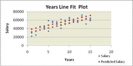
by an average of $2,314. A glimpse at the line fit plot illustrates the above
discussion. This plot is shown in Worksheet 3.3.10. Note the two lines, the top
being the predicted salary line for male faculty, the bottom curve for female
faculty. The salary line is typical in a public university as faculty gets
promoted to associate and then full professor by the 10 - 15 year point. What
should not be typical is the two curves as that is discrimination if all other
factors are the same. Parallel lines are indicative of no interaction among the
independent variables confirming the findings of our first test in this
example. No matter the degree of
experience, males will make in the average $6,733 more than females, and we say
that the relationship between salary and years of experience is not dependent
upon gender.
Worksheet 3.3.10
Practical Utility
The adjusted R Square
is approximately 0.67 meaning that years experience and gender explain 67% of
the sample variation in salary in this straight line model. This is a moderate
degree of explained variation. This explanatory power could be increased if we
attempted to model a curvilinear relationship between salary and years of
experience. Note that the actual data plot appears to indicate that a curvilinear
model would be a better predictor of salary than the straight line model. This same interpretation can be inferred from
the error plot in Worksheet 3.3.11.
However, we'll let this issue for another more advanced course and
continue with our analysis as we initially hypothesized the model. The Standard Error of the Model is $7,482
which is interpreted to be 95% of the actual salaries will be within +/- 2 *
$7,482 or +/- $14,964 of the predicted salaries. This error is obviously too
high for prediction purposes, but if the model was to be used solely to
understand the discrimination effect, it might be acceptable. I should add a
caution here. You may have noticed that there were just 30 observations in this
example. There should have been a minimum of 50. If we used the larger minimum
number of observations, the standard error should improve (remember standard
errors and standard deviations reduce as you increase sample size to the
minimum required).
Statistical Utility
The following hypothesis test is used to determine model utility.
H0:
B1 = B2 = B3 = 0 (regression model is not
statistically useful)
Ha: At least one B =/= 0 (model is statistically useful)
Since the p-value (1.46E-07)
for the F statistic in the Regression Row of the ANOVA table of Worksheet 3.3.9
is less than alpha of 0.05, reject the null hypothesis and conclude that the
model is statistically useful.
Assumptions
I examined the standardized residuals and the normal probability plot and
found no outliers, indicating that the assumption that the error terms are
normally distributed around a mean of zero can be considered met. To determine
if we meet the assumptions that the error has constant variance and is
independent, we examine the residual plots.
There will be two plots of interest, the plot for the quantitative X and the
plot for the qualitative X. You will also get a plot for the curvature term but
this is a derived variable and may be ignored. Assignment 3, Step 5, in the
Main Module 3 Notes and repeated at the beginning of this note set states
exactly what residual plots you need according to which model number is your
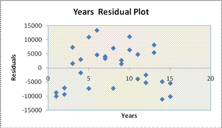
best model. Worksheet 3.3.11 provides the residual plot for Years, and
Worksheet 3.3.12 provides the residual plot for gender.
Worksheet 3.3.11
Worksheet 3.3.12
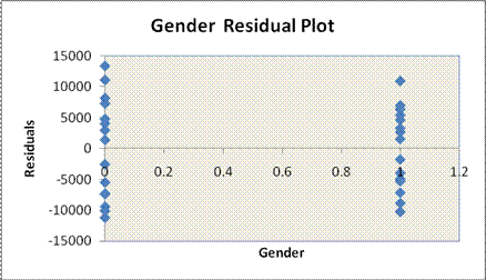
The Years Residual Plot shows negative error for small and large values of
experience compared to the middle range (between 5 and 10 years). This is an indication that a curvilinear model
would be a better model to meet our assumption of constant variance and random
distribution of errors. Again, we will leave the curvilinear model analysis for
another course. As well, the male gender
residual is smaller than the female residual. This is a second indication of a
small sample size problem. A larger sample size should even out the
distribution of the error for all values of the independent variables.
Making a Prediction
To predict the salary for the first female faculty member in our data set
(13 years experience), we first obtain the point estimate:
Eq.
3.3.9: Salary = 29752 + 2314 Years + 6733 Gender
Salary = 29752 + 2314 (13) + 6733 (0)
Salary = $59,834
Next, incorporate the standard error to get a 95% prediction interval:
Eq. 3.3.10: Salary = 59834 +/- (2 * 7482) = 59834 +/- 14964.
So,
we are 95% confident that a female faculty member with 13 years experience will
make between $44,870 and $74,798. As indicated earlier, that is a wide range
for prediction purposes. Perhaps more data or stratification of the faculty by
years of experience would produce a model with less error.
The error of prediction for this particular observation is actual minus
predicted which is 68,000 - 59,834 or $8,166.
Next, we run the regression analysis with residual output, residual plot, line
fit plot, and normal probability plot. These are used to evaluate practical
utility, statistical utility, the assumptions, and to make the prediction.
That's it. I hope these two examples provide a "feel" for model
building.
References:
Anderson, D., Sweeney, D., & Williams, T. (2006). Essentials of Modern Business Statistics with Microsoft Excel. Cincinnati, OH: 3rd Edition , South-Western, Chapter 13.
Ken Black. Business
Statistics for Contemporary Decision Making. Fourth Edition, Wiley.
Chapter 13, 14, 15 (Advanced chapter: 16)
D. Groebner, P.
Shannon, P. Fry & K. Smith. Business
Statistics: A Decision Making Approach, Fifth Edition, Prentice Hall, Chapter 12 & 13
Sheskin, David J. (2000). Handbook of Parametric and Non
Parametric Statistical Procedures (2nd. ed.). Boca Raton, FL: CRC
Press LLC, Test 28.
Levine, D., Berenson, M. & Stephan, D. (1999). Statistics for Managers Using Microsoft Excel (2nd. ed.). Upper Saddle River, NJ: Prentice-Hall. Chapter 14 -- Multiple Regression Models
Mason, R., Lind, D. & Marchal, W. (1999). Statistical Techniques in Business and Economics (10th. ed.). Boston: Irwin McGraw Hill. Chapter 13 -- Multiple Regression and Correlation Analysis
| Return to Module Overview | Return to top of page |
|
|