|
‘Let's
take flight simulation as an example. If you're trying to train a pilot, you
can simulate
almost the whole course. You don't have to
get in an airplane until late in the process.’
Roy
Romer
4.1 Simulation
Simulation studies enable an
objective estimate of the probability of a loss (or gain) which is an important
aspect of risk analysis. One of the main
advantages of simulation over analytical models is the ability to use
probability distributions that are unique to the system being studied. This ability gives the user the opportunity
to model complex system behavior which would be very difficult or even
impossible to do with analytical models.
Simulation models are flexible; they can be used to describe systems
without requiring the assumptions that are often required by mathematical
models. Another advantage is that
simulation model will provides a convenient experimental laboratory for the
real system. But simulation is not
without disadvantages. The process of
developing, verifying and validating large complex system can be costly and
time consuming. Also, simulation run
only provides a sample of how the real system will behave; that is, the results
of a simulation run only provides estimates or approximations about the real
system. Consequently, simulation does
not guarantee an optimal solution. However, the chances of obtaining poor
solution is mitigated if the analyst
uses good judgment in developing the
model and the simulation process is run long enough and under different
conditions so that the analyst has sufficient data to predict hoe the real
system will operate.
Before we start the basics of
simulation and do some practical examples, read Chapter 12, Q.M in Action 'Call
Center Design'. Appreciate how simulation
is used in many types of businesses and functions within an organization. In reality, with advancements in computer
technology, simulation has rapidly replaced many analytical models we cover in
this and other management science courses.
In the near future, with the costs of technology decreasing and further
advancements in the area of real time information (and wireless communication),
I expect that simulation will be part of everyday operations, anticipating
events and planning production and services to meet customers satisfaction on a
continual basis. Some of the more
‘enlightened’ companies already continuously collect data from thousands or
even millions point-of-sale (POS) terminals and feed that information to
specialized simulation software as part of what lately is called business
intelligence systems. All major
corporations already depend on simulation to run complex business operations
around the globe to optimize their supply chain, diminish the risk of
disruption and increase safety in the delivery process.
4.1.1 Generating Simple Random Numbers
with Excel
An essential
part of simulation procedure is the ability to generate representative values
for the probabilistic inputs. Let’s
review how to generate these values. One
simple way (the old fashion way) is to use random number tables that can be
used to select a random number. Another way (now that we have easy access to
computers) is to use Excel random number generators to accomplish this task, or
any random number generator presented in several software packages. In Excel, the function =RANDBETWEEN(a,b) returns a random integer
number between the numbers a and b you specify. A new random
integer number is returned every time the worksheet is calculated (‘Enter’ or
F9 key is pressed).
Syntax:
=RANDBETWEEN(a,b)
a:
is the smallest integer RANDBETWEEN will return.
b:
is the largest integer RANDBETWEEN will return.
Example: =RANDBETWEEN(1,100)
returns a random number between 1 and 100.
Application:
There are 48 names in the list presented in figure 4.1. Each student is associated with an ordinal
number from 1 to 48 and we need to select one at random. By inserting the function =RANDBETWEEN(1,48) into an Excel cell it returned the value 44.
That means Stephanie (associated with number 44) was randomly selected from her
class.
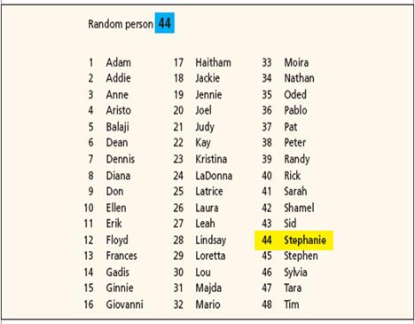
Figure
4.1
The Excel
function RAND() is very useful in many applications to
generate random numbers. It returns an evenly distributed random real number (from a Uniform
Distribution) between 0 and 1. A new random real number is returned every time
the worksheet is calculated or F9 key is pressed.
Syntax:
=RAND( )
With this function,
we can generate inputs to many simulation models where a uniform distribution
is required.
·
To
generate a random real number between a and b, use:
=RAND()*(b-a)+a
·
To
generate a random number between 0 and 100, use
=RAND()*100
If you want to
use RAND to generate a random number but don't want the numbers to change every
time the cell is calculated, you can enter =RAND() in the formula bar, and then
press F9 to change the formula to a random number. See an example here.
Some
computers may recalculate the content of a cell every time you press Enter key.
That is, the random number generator will update the content of a cell having
the function =Rand() with a new random number. To stop this feature you have to deactivate
the auto calculation. See how to do it
through this
video.
Generating
random numbers is a very flexible technique to model many types of
distribution; Uniform, Normal, Exponential, Poisson (seen in Line Management
Module), and others presented in many business processes. Refer to the textbook for additional
explanation of random numbers and how to generate probabilistic input values
(including how to use Rand() function to obtain a
value from a probabilistic input that has a symmetric ‘bell’ shape
distribution.)
Next, let us
see how random numbers is an integral part of simulation by learning an
application of simulation in risk analysis.
4.1.2 Application: Waiting
Line Simulation
Review the chapter to learn
how we can model waiting lines and contrast with the analytical model for Ocala
Software Systems – problem 14 (13th edition). Remember that already we worked with Poisson
and Exponential distributions to model customer arrival and service times. Pay attention to important concepts such as
Static versus Dynamic simulation, Event and Discrete-event simulation,
Verification and Validation of a model.
The following are important distributions using random numbers for line
management simulation:
= NORMINV(RAND(),m,s)…normal distribution with mean m and standard deviation s.
=
- (1/λ)*LN(RAND())…Poisson distribution for an
arrival rate λ
= -
μ*LN(RAND())…Exponential distribution with mean service time μ. Pay
attention that in this formula we use mean service time, and not the mean
service rate in line management.
Let’s see an
application. Ocala software operates a
technical support office and wants to know the operating characteristics of the
call center used by its customers for consultation. The following is the
information given in the problem:
(for additional data please see Problem 14, Ocala Software
Systems (page 531 – 13th edition) call center problem)
Number of channels: 1
Arrival
rate is 5 calls per hours à lambda =
λ = 5
Service
rate is 8 callers per hours à mean
service time = µ = 7.5 minutes or 0.125 hours
A simulation
has to account for the 3 stages that take place when a call arrives at the call
center:

Therefore we have to create a
spreadsheet that replicates what happens in each stage of the simulation.
|
Inter-arrival |
Arrival |
Waiting |
Start |
Service |
End |
|
|
Customer |
Time |
Time |
Time |
Time |
Time |
Time |
|
1 |
0.06 |
0.06 |
0.00 |
0.06 |
0.06 |
0.12 |
|
2 |
0.02 |
0.08 |
0.03 |
0.12 |
0.14 |
0.26 |
|
3 |
0.24 |
0.32 |
0.00 |
0.32 |
0.04 |
0.36 |
Let us use customer 2 to
explain the details:
Inter-arrival time is a
random process modeled through a random function such as - (1/λ)*LN(RAND()). We use
this specific function because the problem indicated that the arrival process
follows a Poison distribution. Had the
problem indicated the arrival process follows a uniform distribution, we would
have to use the corresponding random function for uniform distribution. The inter arrival time is just the time
between arrivals (in practice this is easy to measure and the consultant build
a histogram after a series of measurement check against a known shape to arrive
at the specific distribution of the arrival process). Customer 2 arrived 0.02
hours ( or 1.2 minutes) after customer 1, and customer
3 arrived 0.24 hours (or 14.4 minutes) after customer 2. Remember that time is
measured in hours in this problem.
Arrival time: It is the clock time the customer arrived at
the call center. It is sequential. If we
assume the office was open at a theoretical time of 00.00 hours, then customer
1 arrived at 0.06. After 0.02 hours,
customer 2 arrived for a total clock time of 0.08. Therefore, arrival time for
customer k is just the previous arrival time (for customer j) plus the
inter-arrival time of customer k.
Waiting time: For customer 2 is 0.03. When this
customer arrived at time 0.08, the technician is busy with customer 1 until
0.12 (see End Time column). Therefore, for
customer k, this waiting time is just the maximum value between end time for
customer j and the arrival time for customer k.
Start Time: is just the
arrival time plus the waiting time. For
customer 2, it arrives at 0.08, waits for 0.03 hours and start at 0.12 hours.
Exponential
service time with mean time µ. It is modeled through the exponential
distribution function given by - μ*LN(RAND()). If the problem had indicated another type of
distribution, we would have to use a different function. Customer 2 took 0.14 hours during the
consultation with the technician.
End time: when the customer leaves the system. It is just the start time plus service
time. For customer 2, it started at 0.12
hours, took 0.14 hours ‘talking’ with the tech person, and left the system at
0.26 hours.
We can replicate the same
stages for many customers to simulate a day of operation, for example. Let us replicate the same stages for 1000
customers and arrive at the following (note that lines 11 to 994 have been omitted):
|
Inter-arrival |
Arrival |
Waiting |
Start |
Service |
End |
|
|
Customer |
Time |
Time |
Time |
Time |
Time |
Time |
|
1 |
0.06 |
0.06 |
0.00 |
0.06 |
0.06 |
0.12 |
|
2 |
0.02 |
0.08 |
0.03 |
0.12 |
0.14 |
0.26 |
|
3 |
0.24 |
0.32 |
0.00 |
0.32 |
0.04 |
0.36 |
|
4 |
0.51 |
0.83 |
0.00 |
0.83 |
0.09 |
0.91 |
|
5 |
0.02 |
0.84 |
0.07 |
0.91 |
0.01 |
0.92 |
|
6 |
0.03 |
0.87 |
0.05 |
0.92 |
0.20 |
1.12 |
|
7 |
0.15 |
1.02 |
0.10 |
1.12 |
0.05 |
1.17 |
|
8 |
0.69 |
1.72 |
0.00 |
1.72 |
0.14 |
1.86 |
|
9 |
0.06 |
1.77 |
0.08 |
1.86 |
0.00 |
1.86 |
|
10 |
0.03 |
1.81 |
0.05 |
1.86 |
0.03 |
1.89 |
|
995 |
0.41 |
200.79 |
0.00 |
200.79 |
0.15 |
200.94 |
|
996 |
0.07 |
200.86 |
0.08 |
200.94 |
0.03 |
200.97 |
|
997 |
0.13 |
200.99 |
0.00 |
200.99 |
0.14 |
201.13 |
|
998 |
0.22 |
201.21 |
0.00 |
201.21 |
0.27 |
201.48 |
|
999 |
0.06 |
201.27 |
0.21 |
201.48 |
0.27 |
201.75 |
|
1000 |
0.16 |
201.43 |
0.32 |
201.75 |
0.06 |
201.81 |
|
0.17* |
|
0.12** |
0.29*** |
|||
|
587 |
58.7% |
|||||
|
41.3% |
||||||
|
511 |
51.1% |
Now we can compute some of
the characteristics of the call center.
*The average waiting time is
0.17 hours, or 10.2 minutes.
** The average service time
is 0.12 hours matching the ‘theoretical’ service time given in the problem.
*** The average time in the
system for a customer is 0.29 given by the average waiting time plus the
average service time (0.17+0.12).
If we count how many
customers had to wait and divide by 1000, we get the probability the customer
has to wait in line. In our example, we had 587 customers with a waiting time
greater than zero (had to wait) and therefore it represents 58.7% of our
simulation. Conversely, there is a 41.3%
probability that the customer will not have to wait for service.
We can conduct additional
analysis to verify the performance again a desired service level. For example, management could indicate the
desired service standards to be a maximum of 10% of customers waiting more that 2 minutes. In
our example, we counted 511 customers waiting longer than the specified and
therefore 51.1% of the customers, well above the service levels required by
management.
Download the Excel file and
inspect the simulation example (just remember that the file may contain
different values form the one indicated here but the overall characteristics –
such as average waiting time, should be approximately equal: OCALA-CALL-CENTER-SIMULATION
It is interesting to compare
the results above from simulation (dynamic) with the analytical (static) model
we cover in the line management chapter.
Here is the result using The Management Scientist software.
WAITING LINES
*************
NUMBER OF
CHANNELS = 1
POISSON
ARRIVALS WITH MEAN RATE = 5
EXPONENTIAL
SERVICE TIMES WITH MEAN RATE = 8
OPERATING
CHARACTERISTICS
-------------------------
THE PROBABILITY OF NO UNITS IN THE
SYSTEM 0.3750
THE AVERAGE NUMBER OF UNITS IN THE
WAITING LINE 1.0417
THE AVERAGE NUMBER OF UNITS IN THE
SYSTEM 1.6667
THE AVERAGE TIME A UNIT SPENDS IN THE
WAITING LINE 0.2083
THE AVERAGE TIME A UNIT SPENDS IN THE
SYSTEM 0.3333
THE PROBABILITY THAT AN ARRIVING UNIT
HAS TO WAIT 0.6250
4.2
Risk Analysis
Start
this section by reading Section 12.1 Risk Analysis and understand 'PortaCom Project' example.
This illustrated example gives you a good review of risk analysis and
one of the approaches called what-if analysis.
In case you missed the definition, risk analysis is just the process of
predicting the outcome of a decision in the face of uncertainty. The value of the ‘uncertainty’ is the random
number you generate and insert in the model for final computation. Pay attention to key concepts such as
parameters, base-case scenario, worst- and best-case
scenarios. Pay attention to figures
12.2, the 'business' model you want to simulate. You should review figure 12.6 and load PortaCom Project spreadsheet available in your CD ROM and
understand the layout and solution of the simulation. Remember that F9 key will perform additional
run of the model. Worksheets for all simulation examples presented in this
chapter are available in the CD ROM that accompanies the text.
4.2.1 Application of What-if Analysis
(in construction)
The following is the Excel
input for the Porta-Com Project described in section
12.1 of the text. Remember that What-If-Analysis allows us to compare scenarios
which are static in nature since there are no probabilities associated with the
outcomes. The parameters of the profit
function have been modified to get another perspective. See if you arrive at the
profit for the best-case scenario. The
Excel file for this example can be downloaded here: PC-risk-analysis

4.2.2
Porta-Com Project Simulation
When the probabilities
associated with the scenarios are known when can refine the what-if analysis to
include risks in the model analysis (we already did this when we studied
Decision Analysis with Probabilities. Remember
that the expected value (EV) approach includes a measure of probabilities in
the computations.) The following is the data/parameters for the problem:

Note how the direct labor
COST distribution is arranged in a table for reference in conjunction with
lower and upper random number interval limits.
The random number will be called in the simulation by =RAND(). If the result of a trial for =RAND()
is 0.7666, then the cost entered in the profit function is $58. Similarly, part costs are the results of
the random function
=a +RAND()*(30),
where 30= a-b = 110-80; and a is the
lowest value for part cost and b the
highest. The ramdom
function for part cost is then given by:
= 80+RAND()*30. If for one trial the result for +RAND() is 0.64, the part will have a cost (random) of $99.20
Since the demand can only
have integer values, the random simulation can be accomplished using =RANDBETWEEN(a,b) where a is the worst-case and b the best-case scenario. The function
entered in the simulation is then given by =RANDBETWEEN(9000,18000).

The simulation trials can be
set up as shown in the figure below.
Note some rows have been omitted.
The profit function is still the same as illustrated in the
what-if-analysis
Profit = (selling price –
cost of labor – cost of material)*demand – administrative costs
Profit
= (229- labor – material) demand – 795,000
However, labor, material
and demand now have a probabilistic nature analyzed through simulation.
Download the Excel file porta-com-simulation-II
and inspect how the
simulation is set up. The economic and
risk analysis are indicated in the last few rows.

Do the following problems to
help you understand this chapter:
P2, P5, P9,
and P14.
You can find the answers in solution and the Excel
simulation for problem 14 (Madeira Manufacturing Co.). You should be ready to tackle the assignment
for Module 4.