HURRICANE DAMAGE GRADIENTS AND VEGETATION COMMUNITY DYNAMICS
To those who study her, Nature reveals herself as extraordinarily fertile and ingenious in devising means, but she has no ends which a human mind has been able to discover or comprehend. Joseph Wood KrutchINTRODUCTION
The pattern of succession following disturbance has been studied for a variety of natural and anthropogenic disturbances. Richards (1953) defined the issues surrounding succession in the tropics as knowing: 1) the changes in soil and vegetation following the removal of primary forest, 2) whether secondary forests will reconstruct the primary forest, and 3) the time required for recovery. Now, 40 years later, these issues remain the focus of study, with two additional ones. What seems to distinguish succession in the tropics from succession in the temperate regions is a more complex suite of possible vegetation responses to disturbance (Richards 1953, Ewel 1980, Hartshorn 1980). The issue then becomes: what environmental and biotic factors affect the particular path to, and rate of, recovery from a given disturbance at a specific site? Much of the focus on this issue has been gap dynamics (Hartshorn 1978, Hubbell & Foster 1986, Denslow 1987, Whitmore 1989a). The second additional issue involves delineating the differences between 'natural' and anthropogenic disturbance (Gomez-Pompa et al. 1972, Uhl 1982, Brown & Lugo 1989, Clark 1990, Whitmore 1991). Hurricanes, like other types of wind disturbance, may result in any of four vegetation responses: 1) regrowth, 2) recruitment, 3) release, and 4) repression (Everham 1995). Although these responses have been reported singly or in combination for all types of wind disturbance (see Chapter 1), little progress has been made toward developing models that can predict the principal path under various conditions. Everham (1995) proposed a two-dimensional gradient space of measures of hurricane damage severity to differentiate between regrowth and recruitment, between recovery dominated by sprouting of surviving stems and recovery through the establishment of early successional species (Chapter 1, Figure 12). The two dimensions of damage are: 1) compositional (percent mortality), and 2) structural (percent stems or percent basal area damaged). These two gradients are secondary, and are used instead of the primary gradients of abiotic factors, to which they are assumed to be correlated. In this chapter I examine the response of vegetation communities to gradients of hurricane damage. First, does position in a two-dimensional gradient space of compositional and structural damage have predictive ability in distinguishing among paths of response? Second, if this predictive ability exists, is it scale independent? Moreover, can damage severity at small spatial scales (down to a 5 m radius circular plot) be used to predict vegetation response and does this relationship hold for larger spatial scales up to tens of hectares?METHODS
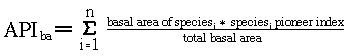
To examine the vegetation response to hurricane disturbance, I remeasured plots in the BEW and the HRP during the fourth year after the hurricane. All of these plots had previously identified and permanently tagged stems (Zimmerman et al. 1994, Scatena & Lugo in press). In the BEW, 83 five meter radius circular plots were established before Hurricane Hugo, on a 40 m grid across the watershed, at differing topographic positions. These plots were resampled within six months after the hurricane to establish hurricane damage severity. I resampled 25 of these plots a second time during the fourth year of recovery (Figure 22a). The HRP was established during the second year of recovery following Hugo. All stems 10 cm dbh and larger were tagged, measured, identified, and assessed for hurricane damage. Voucher specimens are stored at the EL Verde Field Station (Zimmerman et al. 1994). During the fourth year after the hurricane I resampled a subset of 18 plots, using a topographically-stratified random sample of the 400 20 m by 20 m quadrats in the HRP (Figure 22b). To allow comparison to the BEW data set, these plots were sampled using a 5 m radius plot centered in each of these 20 m by 20 m quadrats. The entire HRP was resampled during the fifth year of recovery and all stems 1 cm dbh or larger were identified, measured, and tagged. The nesting of the circular plots within the quadrats in the HRP allows placement of the plot within the damage gradient space at two different scales. Damage severity, measured as compositional and structural damage, may be quantified based on the stems within the circular plot or within the entire 20 m by 20 m quadrat. Figure 22 - Locations of sampling points, chosen to represent topographic positions of: ridges, slopes, benches (only in the HRP), and valleys. A. Bisley Experimental Watershed B. Hurricane Recovery Plot. Calculation of API - Whitmore (1989b) introduced the use of the "average pioneer index" (API) as a measure of community composition to track recovery of the Kolombangara rain forests, Solomon Islands. This index was calculated using the ratio: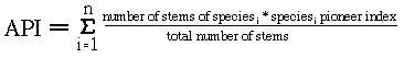 Whitmore's pioneer index is a categorical variable with values
ranging from 1 to 4, most shade-tolerant to least shade-
tolerant, respectively. The assignment of each species to a
category was based on previous studies of seedling dynamics
(Whitmore 1974), and assumes that shade tolerance is an index
of successional position. For the LEF, I use two categories:
late successional and early successional species (1 and 2,
respectively). The use of only two categories follows the work
of Zimmerman et al. (1994) who found two distinct categories of
tree species response to hurricane disturbance. The
assignments to a given category are based on recognized
distributions under different stages of recovery (Little &
Wadsworth 1964, Crow & Weaver 1977, Weaver 1983), shade
tolerance (Smith 1970), comparative measures of seedling
frequencies, seed size, and wood density (Weaver 1992),
measured occurrence of seedlings under different light
conditions (Devoe 1989), and the assessment of each species by
researchers familiar with the LEF (F. Scatena, personal
communication; C. Taylor, personal communication).
I determine mean pioneer index for each plot after three
years of recovery, using Whitmore's equation and the following
modification based on basal area:
Whitmore's pioneer index is a categorical variable with values
ranging from 1 to 4, most shade-tolerant to least shade-
tolerant, respectively. The assignment of each species to a
category was based on previous studies of seedling dynamics
(Whitmore 1974), and assumes that shade tolerance is an index
of successional position. For the LEF, I use two categories:
late successional and early successional species (1 and 2,
respectively). The use of only two categories follows the work
of Zimmerman et al. (1994) who found two distinct categories of
tree species response to hurricane disturbance. The
assignments to a given category are based on recognized
distributions under different stages of recovery (Little &
Wadsworth 1964, Crow & Weaver 1977, Weaver 1983), shade
tolerance (Smith 1970), comparative measures of seedling
frequencies, seed size, and wood density (Weaver 1992),
measured occurrence of seedlings under different light
conditions (Devoe 1989), and the assessment of each species by
researchers familiar with the LEF (F. Scatena, personal
communication; C. Taylor, personal communication).
I determine mean pioneer index for each plot after three
years of recovery, using Whitmore's equation and the following
modification based on basal area:
 Comparison of Gradient Approaches - API can be calculated
two ways, can be based on data from either the 20 m square
quadrat or the 5 m radius plot, and can utilize a minimum stem
size of 1 cm, 4 cm, or 10 cm at either spatial scale. Any
method of calculating API can be related to hurricane damage
measurements at either spatial scale (5 m or 20 m). Therefore,
I compare: 1) quantifying API (using stems or using basal
area), 2) quantifying structural damage using either percent
stem damage or percent basal area damage, 3) vegetation
response at spatial scale of 5 m or 20 m plot using minimum
stem sizes of 1 cm, 4 cm, or 10 cm, and 4) quantifying damage
at a spatial scale of 5 m or 20 m. Separate analyses were run
to compare all possible combinations of the above approaches.
In each case, the plots were located in a gradient space
of compositional damage and structural damage and the best line
placed through the space to separate plots with API of less
than 1.33 and those greater than 1.33. This API value was
selected as a natural break in the distribution of pre-
hurricane API values for the plots in the HRP (Figure 23), and
represents a plot where at least one third of the stems (or the
basal area) are early successional tree species. The percent
error was calculated as the percent of plots with API less than
1.33 that were located incorrectly above the line and plots
with API greater than 1.33 incorrectly located below the line.
Figure 23 - Distribution of Average Pioneer Index values for
the 18 Hurricane Recovery Plots, before Hurricane Hugo, based
on the assessment of 10 cm stems. Results presented for both
equations, based on stems or basal area.
Comparison to Indirect Gradient Approaches - I also
compared API to other measures of community composition:
principal component analysis (PCA) and polar ordination (PO).
Both PCA and PO are indirect gradient analysis techniques. The
species data is used to arrange or order the plots, and the
order can be compared to potential explanatory environmental
gradients, a posteriori. These two analyses were performed
using the programs developed by Ludwig and Reynolds (1988),
PCA.BAS and PO.BAS.
PCA (used in Chapter 2 to analyze patterns of abiotic,
biotic, and damage measures) is an eigenanalysis ordination
method. The correlation matrix of species counts is
partitioned into axes, each of which corresponds to an
eigenvalue of the matrix, the variance of the data accounted
for by the axis (Ludwig & Reynolds 1988). PCA was first
applied to ecological matrices by Goodall (1954).
The PO method of Bray and Curtis (1957) was developed to
analyze plant community data. In this analysis, plots are
placed within a coordinate system where their relative
similarities are reflected by their proximity. Ludwig and
Reynolds' program uses the endpoint selection following the
original techniques described by Bray and Curtis (1957), and
only calculates the first two dissimilarity axes. The
dissimilarity measures are calculated as euclidean distances
(Ludwig & Reynolds 1988).
Testing Direct Gradient Approach - The most effective
approach to developing an isopleth for distinguishing between
the recovery vectors of regrowth and recruitment, (which were
defined by mean pioneer index) is determined for the 18 plots
of the HRP. Additional plots are selected from the 400 20 m
quadrats of the HRP, based on their damage severity, to refine
the position of the isopleth. Then, the predictive ability of
these positions in gradient space is tested in two ways and at
two spatial scales. I then test the isopleths for their
ability to predict community dynamics, (i.e. presence of early
or late successional species), in 100 other randomly selected
20 m by 20 m quadrats. These relationships then are examined
at the smaller spatial scale, based on the 5 m radius circular
plots in the BEW.
Comparison of Gradient Approaches - API can be calculated
two ways, can be based on data from either the 20 m square
quadrat or the 5 m radius plot, and can utilize a minimum stem
size of 1 cm, 4 cm, or 10 cm at either spatial scale. Any
method of calculating API can be related to hurricane damage
measurements at either spatial scale (5 m or 20 m). Therefore,
I compare: 1) quantifying API (using stems or using basal
area), 2) quantifying structural damage using either percent
stem damage or percent basal area damage, 3) vegetation
response at spatial scale of 5 m or 20 m plot using minimum
stem sizes of 1 cm, 4 cm, or 10 cm, and 4) quantifying damage
at a spatial scale of 5 m or 20 m. Separate analyses were run
to compare all possible combinations of the above approaches.
In each case, the plots were located in a gradient space
of compositional damage and structural damage and the best line
placed through the space to separate plots with API of less
than 1.33 and those greater than 1.33. This API value was
selected as a natural break in the distribution of pre-
hurricane API values for the plots in the HRP (Figure 23), and
represents a plot where at least one third of the stems (or the
basal area) are early successional tree species. The percent
error was calculated as the percent of plots with API less than
1.33 that were located incorrectly above the line and plots
with API greater than 1.33 incorrectly located below the line.
Figure 23 - Distribution of Average Pioneer Index values for
the 18 Hurricane Recovery Plots, before Hurricane Hugo, based
on the assessment of 10 cm stems. Results presented for both
equations, based on stems or basal area.
Comparison to Indirect Gradient Approaches - I also
compared API to other measures of community composition:
principal component analysis (PCA) and polar ordination (PO).
Both PCA and PO are indirect gradient analysis techniques. The
species data is used to arrange or order the plots, and the
order can be compared to potential explanatory environmental
gradients, a posteriori. These two analyses were performed
using the programs developed by Ludwig and Reynolds (1988),
PCA.BAS and PO.BAS.
PCA (used in Chapter 2 to analyze patterns of abiotic,
biotic, and damage measures) is an eigenanalysis ordination
method. The correlation matrix of species counts is
partitioned into axes, each of which corresponds to an
eigenvalue of the matrix, the variance of the data accounted
for by the axis (Ludwig & Reynolds 1988). PCA was first
applied to ecological matrices by Goodall (1954).
The PO method of Bray and Curtis (1957) was developed to
analyze plant community data. In this analysis, plots are
placed within a coordinate system where their relative
similarities are reflected by their proximity. Ludwig and
Reynolds' program uses the endpoint selection following the
original techniques described by Bray and Curtis (1957), and
only calculates the first two dissimilarity axes. The
dissimilarity measures are calculated as euclidean distances
(Ludwig & Reynolds 1988).
Testing Direct Gradient Approach - The most effective
approach to developing an isopleth for distinguishing between
the recovery vectors of regrowth and recruitment, (which were
defined by mean pioneer index) is determined for the 18 plots
of the HRP. Additional plots are selected from the 400 20 m
quadrats of the HRP, based on their damage severity, to refine
the position of the isopleth. Then, the predictive ability of
these positions in gradient space is tested in two ways and at
two spatial scales. I then test the isopleths for their
ability to predict community dynamics, (i.e. presence of early
or late successional species), in 100 other randomly selected
20 m by 20 m quadrats. These relationships then are examined
at the smaller spatial scale, based on the 5 m radius circular
plots in the BEW.
RESULTS
When damage is quantified using compositional and structural measures, the position within a gradient space of damage can predict the post-disturbance API accurately in 94% percent of plots. This maximum level of predictive ability occurs using the 20 m spatial scale and a minimum stem size of 4 cm. High predictability also occurs when the damage is quantified at a scale of 20 m and the response is predicted for a 5 m plot nested within it (89%). This direct gradient approach is more effective than either polar ordination or principal component analysis in differentiating plots based on API. Calculation of API - A total of 101 species were identified in the 43 plots, including the entire 20 m by 20 m quadrat for the plots in the HRP, and in the additional 100 quadrats used for testing the damage gradient predictions (Appendix C-XI). Of the 101 species, 46 are classified as late successional species and 55 as early successional species. Of the species, 18 are endemic to Puerto Rico, and five are exotics. The 25 plots in the BEW (0.196 ha) included 37 species. The 18 plots in the HRP (0.141 ha) included 45 species (using only the data from the 5 m radius circular plots). 22 species occurred at both sites. For total site values, the BEW has higher stem density, higher basal area, and significantly higher API (APIba is higher, but not significantly so). The higher API for the BEW is consistent for all topographic positions (for definitions of topographic classification, see Chapter 2). The HRP has higher species richness, due principally to a greater number of species in the ridge plots. The HRP ridge plots also have much higher basal area (42.89 m2/ha) compared to the BEW ridge plots (27.05 m2/ha), but the sample size is small (n=4) in both cases. The BEW was more impacted by Hurricane Hugo (mortality = 10.96%, BA damaged = 24.30%, and stems damaged = 15.01%), compared to the HRP (5.98%, 16.55%, 12.82%). Table 15 presents the summary of data from the post-disturbance measurements at both study areas. The individual plot data appears in Appendix C-XII; and the damage and ordination axes values are in Appendix C-XIII. Selecting Gradient Approach - Table 16 summarizes the results of the 32 analyses using different combinations of API quantification, structural damage quantification, spatial scale to quantify vegetation response, minimum stem size, and spatial scale to quantify damage. Comparing all analyses based on the method used to calculate API, stem damage or basal area damage, Whitmore's (1989b) original formula using number of stems results in an average of 64.3% correct. The alternative index based on basal area had an average correct of 54.3% Possibly the use of basal area error over-represents the few large surviving stems in an area dominated by recruitment of early successional species. All subsequent analyses used API calculated using stem counts. Table 15 - Comparison of plot summaries for post-hurricane measurements for each study site. Measurements form the fourth year of recovery from Hurricane Hugo. Average pioneer index based on stems (API) or basal area APIba), and calculated as average of all plots (95% confidence limit). Basal area (BA) reported in square meters. Results based on data only from 5 m radius circular plots, using all stems > 4 cm. Damage assessed on > 10 cm stems only.Summary Characteristic BEW HRP
Number of Plots 25 18 Stems Density (stems/ha) 2772 1784 Basal Area (m2/ha) 38.72 36.51 Percent Mortality 10.96 5.98 Percent Stems Damaged 15.01 12.82 Percent BA Damaged 24.30 16.55 API (95% limit) 1.71 (0.17) 1.38 (0.12) pre-hurricane API 1.15 1.24 APIba (95% limit) 1.48 (0.21) 1.39 (0.11) pre-hurricane APIba 1.14 1.35
Plots on Ridges 4 4 Species on Ridges 14 26 API on Ridges 2.22 1.85 Stem Density (stems/ha) 2771 2165 BA on Ridges (m2/ha) 26.54 40.21
Plots on Slopes 15 6 Species on Slopes 29 24 API on Slopes 2.13 1.60 Stem Density (stems/ha) 2854 1869 BA on Slopes (m2/ha) 40.77 36.99
Plots on Benches 0 4 Species on Benches - 24 API on Benches - 1.65 Stem Density (stems/ha) - 1561 BA on Benches (m2/ha) - 37.72
Plots in Valleys 6 4 Species in Valleys 16 14 API in Valleys 2.13 1.36 Stem Density (stems/ha) 2569 1497 BA in Valleys (m2/ha) 41.73 30.89
Total Species 37 45 Early Successional Species 17 18 Late Successional Species 20 27 Endemic Species 8 8 Exotic Species 2 1
When comparing the use of percent stem damage to percent basal area damage, the latter was expected to show a better predictive ability. Basal area damage emphasizes the damage to large stems which would be expected to have more of an impact on the primary gradients of light and temperature. However, the predictive ability of the respective gradient spaces showed little difference. Damage quantified as basal area resulted in 59.3% correctly placed plots. Damage quantified as stem loss gave 60.5% correct. Table 16 - Comparison of different methods of quantifying Average Pioneer Index at different spatial scales. Proportion of correct identification of plots API, based on position of plots in a gradient space of percent mortality and percent stem damage or percent basal area (BA). All comparisons based on 18 plots in HRP.
Damage Quantification Response Data Sets plot size Data Sets stem size
Plot | Damage Response 5 m 20 m 20 m 20 m Size | Measure (4 cm) (1 cm) (4 cm) (10 cm)
| Percent API 0.50 0.44 0.67 0.67 | Stem 5 m | Damage APIba 0.61 0.50 0.50 0.50 (10 cm)|------------------------------------------------------- | Percent API 0.50 0.44 0.67 0.67 | BA | Damage APIba 0.61 0.50 0.50 0.50
| Percent API 0.89 0.39 0.94 0.72 | Stem 20 m | Damage APIba 0.67 0.56 0.56 0.56 (10 cm)|-------------------------------------------------------- | Percent API 0.78 0.44 0.89 0.67 | BA | Damage APIba 0.61 0.50 0.50 0.50
All possible combinations of spatial scale and minimum stem size were not possible. The minimum stem size used in the 5 m circular plots was 4 cm, so this was the only minimum stem size used for this spatial scale. The 20 m quadrat scale could be analyzed using 1 cm, 4 cm, or 10 cm minimum stem size. The lowest average correct is with a minimum stem size of 1 cm, followed by a minimum stem size of 10 cm, and the highest average correct with a minimum stem size of 4 cm (47.1%, 59.9%, and 65.4% respectively). The l cm stem size may include too many previously established shrubs, or too many early successional stems that are already suppressed by a canopy closing above it. The 10 cm stem minimum may miss the new recruiting stems when the sample is taken four years after the hurricane. Presumably the minimum stem size could be larger with a greater amount of time following the hurricane. Examining the spatial scales of damage quantification and the spatial scale of response quantification allows three comparisons: 1) damage quantified at 5 m scale and response quantified at the same scale, 2) damage quantified at the 20 m scale and response quantified at the same scale, and 3) damage quantified at the 20 m scale but response quantified at the finer 5 m scale. Both of the first two approaches can be impacted by edge effects, damage outside the plot influencing response inside the plot. Presumably the 20 m scale would have less of an edge effect, and this approach resulted in a higher percent correct (60.3% compared to 55.5% when using the 5 m scale for damage and response). Using the 20 m scale for damage and the 5 m scale for response, results in the highest percent correct of the three approaches, 73.6%. Predictive ability of the damage gradient space seems most powerful when the damage is assessed for a larger area, and the recovery plot is nested within this larger area to minimize edge effects. Comparison to Indirect Gradient Techniques - The API approach proposed by Whitmore (1989b) is also compared to community ordination techniques, PO and PCA. The first three principal components of this analysis account for only 23.3% of the variation of the vegetation data. Figure 25 shows the distribution of the plots in the first two principal components and distinguishes between plots with an API greater than 1.33, and between plots from the two study sites. Figure 25 presents the same analysis for polar ordination, distinguishing between plots with greater than or less than 1.33 API and between plots in the HRP versus the BEW. Neither of these two ordination techniques appears to do a good job of separating plots dominated by recruitment of early successional species (API > 1.33), but both do separate plots between the two study sites. The first principal component and the second axis of the PO seem to distinguish between HRP and BEW plots. Figure 24 - PCA of vegetation in all 43 plots. Values for the first two principal components plotted. Figure 25 - Polar ordination analysis of the vegetation data of all 43 plots. Dissimilarity values for the first two ordination axes plotted. Testing the Direct Gradient Approach - Using a damage gradient space of compositional damage and structural damage, Figure 26 shows the distribution of all plots in the HRP, based on data at the 20 m by 20 m quadrat scale. The subset of 18 plots that I selected from a topographically stratified random sample and remeasured for this analysis are delineated. The distribution of these plots extends into the lower left corner of the graph, but the locations on the graph are obscured by the concentration of other points there. Note the concentration of points along the y-axis, representing plots with structural damage, snapped or uprooted stems, but no mortality. The lack of plots with extremely low (but non-zero) percent mortality is the result of the limited number of stems per quadrat. Figure 26 - Location of all 400 quadrats of the HRP in a damage gradients space of compositional damage (percent mortality) and structural damage (percent basal area damaged). Figure 27 shows the distribution of the 18 remeasured plots more clearly. These plots indicated an isopleth from roughly 35% structural damage to 17% compositional mortality that distinguishes between plots dominated by recruitment of early successional species (API > 1.33), and those dominated by regrowth of surviving primary forest species (API < 1.33). This line gives an 11% error in placement of plots, as one plot has an API > 1.33 but occurs below the line and one with an API < 1.33 occurs above the line. These 18 plots were located in the damage gradient space by using the data from the entire 20 m quadrat. An additional 18 plots, selected based on their damage severity to refine this isopleth, are included in Figure 28. The resulting isopleth has the formula: y = -0.021 x3 + 0.2 x2 - 0.65 x + 29.7 This isopleth results in a 22.2% error in the placement of plots; four plots are incorrectly placed above the line and three plots are incorrectly placed below the line. Two of the plots incorrectly located below the line (with an API > 1.33) had an API of greater than 1.33 before the hurricane, and therefore the higher API without high severity of damage could be expected. Figure 27 - Location of subset of 18 plots of the HRP in a damage gradients space of compositional damage (percent mortality) and structural damage (percent basal area damaged). Figure 28 - Location of subset of 18 plots of the HRP and an additional 12 plots used to refine the position of the isopleth of recovery path in a damage gradients space of compositional damage (percent mortality) and structural damage (percent basal area damaged). When this damage gradient space is tested with an additional 100 randomly selected quadrats from the HRP (without replacement of the 18 original plots or the additional 18 plots), 64% of the plots are placed on the correct sides of the damage isopleths (Figure 29). This analysis is based on the data from the entire 20 m quadrat for both damage assessment and recovery. Of the 36 incorrectly placed plots, 35 of them had API > 1.33 but are located below the line. Of these 35 plots, 15 had pre-hurricane API > 1.33, again explaining the higher post-hurricane API without severe damage. If the plots with higher pre-hurricane API are excluded, the number of plots correctly predicted is 75%. Testing this relationship at a smaller spatial scale in the BEW, only 52% of the plots are predicted correctly (Figure 30). In this analysis, both the damage assessment and the recovery quantification are based only on the vegetation within the 5 m radius circular plot. All but one of the plots which are incorrectly placed have an API > 1.33, but occur below the line in the damage gradient space. Many of these plots have assessed compositional and structural damage of 0%. Damage outside of these plots may be affecting the recovery within the plot. At this spatial scale, the predictive ability or the two-dimensional gradient space of damage severity breaks down. Figure 29 - Test of additional 100 quadrats randomly selected form the HRP remeasurement, in a damage gradient space of compositional damage (percent mortality) and structural damage (percent basal area damaged). Damage and response quantified at the 20 m spatial scale. Figure 30 - Location of subset of 25 plots of the BEW in a damage gradient space of compositional damage (percent mortality) and structural damage (percent basal area damaged). Damage and response quantified at 5 m spatial scale.
DISCUSSION
The use of a two-dimensional gradient space of structural damage and compositional damage is effective with (some limitations) in differentiating sites whose recovery is through recruitment of early successional species as opposed to those sites whose recovery is dominated by regrowth of surviving primary forest species. This predictive model is effective on the largest scales in this study (tens of hectares), as it predicts correctly the different overall paths to recovery between the HRP and the BEW, based on the average levels of compositional and structural damage and as quantified by API values above or below 1.33. The model also is effective at the scale of 20 m plots, but fails if the plot data is taken from a finer resolution (5 m). As is indicated in Chapter 2, damage varies at scales as small as 5 m subquadrats. At this fine a spatial scale, plots can be impacted by damage that occurred outside the plot. The failure of the two-dimensional damage gradient space is most often related to plots that recover through recruitment, but are classified as undamaged at this small spatial scale. This predictive model also fails to incorporate the impacts of previous damage. Many plots are incorrectly predicted to recover by regrowth due to low damage, but have high densities of early successional species that were established before the hurricane, presumably due to previous disturbance. If this pre-hurricane disturbance history can be included in the analysis, the predictive ability of the model increases. It might be particularly effective to consider the change in API resulting from different positions in the gradient space. Finally, the role of biota in influencing the vector of response is not incorporated. It is probably more realistic to view the position in this damage gradient space as indicating the conditions for vegetation response. The actual post- disturbance vegetation dynamics must be partly influenced by the available propagules. If seeds of early successional species are not available, or are unable to germinate; or the seedlings cannot establish themselves; recovery through the recruitment process will not occur. This analysis is based on differentiating the two recovery paths using Whitmore's API, rather than more commonly used community ordination techniques, such as PCA and PO. Both PCA and PO fail to distinguish between plots with high and low API. PCA gives equal weight to rare or common species in the correlation matrix. In the analysis of all 43 plots, the first principal component is loaded most heavily by Buchenavia capitata, Drypetes glauca, Eugenia stahlii, Sloanea berteriana, Tabebuia heterophylla, and Zanthoxylum martinicense. All but the last two are late succesional forest species, but the most common late successional species, Dacryodes excelsa, is not loaded heavily on this principal component. The second principal component is loaded most heavily by the species: Byrsonima spicata, Casearia arborea, Poutera multiflora, and Homalium racemosum. These four species are a mixture of early and late successional species, but again the most common late successional species and the most common early successional species, Cecropia schreberiana, have little impact on separating the plots. PCA identifies the species that distinguish among plots and will therefore emphasize rarer species. This tends to separate the two study areas whose geographic separation results in some differences in the distribution of rarer species. PO, in part, accounts for these rare species in the calculation by incorporating only the species that occur in both sites for determining the numerator for each pairwise comparison. However, species with similar roles in succession are still treated independently, and the ordination fails to separate the plots based on proportion of early successional species. Figure 31 - PCA of all 43 plots with species pooled into categories based on successional classes. If all species are pooled into the two successional classes and PCA is applied to all 43 plots, (Figure 31), the plots dominated by regrowth (API < 1.33) are clustered mostly in the center of the graph. The first principal component partly separates the plots based on the study area. Although this analysis distinguishes between the two paths to recovery, the equations for the principal components are based on the combinations of species present and their ability to account for variance in the data set, are site specific, and therefore are not able to be translated to another site. In contrast, API can be calculated for any site whose species can be classified into categories of early and late succession and therefore this approach can facilitate the development of more robust models that can be applied among sites with different vegetation communities. The use of a two-dimensional gradient space of hurricane damage is effective in predicting the paths of recovery as defined by the API of the recovering site, at appropriate spatial scales, and particularly if pre-hurricane community data is available. If data on landscape patterns of damage severity are available, or can be modeled accurately based on site data, this analysis can be applied to modeling the vegetation community dynamics during recovery.Return to the Table of Contents