|
Index to Module 4 Notes
|
In Module Notes 4.4, we
introduced ANOVA as a powerful tool that allows us to compare samples of
multiple groups and make conclusions concerning the equality of the population
mean on one dimension or factor. The example we used was comparing mean mile
per gallon performance (the outcome measure) for automobiles tested with
different brands of gasoline (the factor). The factor, brand of gas, has three
levels, Brand A, B and C.
In this set of notes, we expand the ANOVA concept to the examination of
situations involving two factors. In the above example, perhaps we want to test
mean mile per gallon performance for automobiles tested with different brands
of gasoline (factor A) as well as different driving conditions (factor B). The
different driving conditions might be city versus highway driving.
In this scenario, if there was a significant brand effect, then we would know
that mean mpg performances groups differ with respect to at least two of the
the three levels of the brand factor. Likewise, if there was a
significant driving condition, then we would know the mean mpg performances
differ with respect to the two levels of the driving condition factor.
But wait a minute, you say! Back in multiple regression when we had two
independent variables, we also were concerned about interaction. Same
thing holds true in Two- Factor ANOVA. Interaction here would mean that we
would have to be concerned about mean mpg performance at six combination
levels of the brand and driving condition factors. That is, mean mpg for city
driving with Brand A, mean mpg for city driving with Brand B, mean mpg for city
driving with Brand C, mean mpg for highway driving with Brand A, mean mpg for
highway driving with Brand B, and mean mpg for highway driving with Brand C.
That's the idea - I want to present two example situations, one with
interaction, and one without.
A
Situation with Interaction
This example is from
a utility company that was experimenting with variable pricing. Two factors are
involved. The first is the length of the peak period. At the long peak
situation (7 am - 7 p.m.), customers would have a 12 hour discount period between
7 p.m. and 7 am. At the short peak situation (8 am - 5 p.m.), customers would
enjoy a 14 hour discount period between 5 p.m. and 8 am. The other factor is
ratio of the discount. A low ratio is approximately a 2:1 discount on rates
during off-peak usage. A high ratio is approximately a 3:1 discount on rates
during off-peak usage.
The company prepared a satisfaction survey and measured satisfaction on a 50
point scale (50 being high satisfaction, 0 being low). The scores for a trial
run of the survey are shown in Worksheet 4.5.1.
Worksheet 4.5.1
|
Low Ratio |
High Ratio |
|
|
Long Peak |
25 |
24 |
|
Long Peak |
26 |
25 |
|
Long Peak |
28 |
28 |
|
Long Peak |
27 |
26 |
|
Short Peak |
22 |
30 |
|
Short Peak |
25 |
26 |
|
Short Peak |
20 |
31 |
|
Short Peak |
21 |
27 |
Worksheet 4.5.1
presents the data as you would enter it in an Excel Worksheet in preparation
for running a Two-Factor ANOVA.
To run the ANOVA, select Tools from the Standard Toolbar, then Data
Analysis from the pulldown menu, then ANOVA: Two-Factor with Replication.
(In Excel 2007 select Data, then Data Analysis. From the pulldown menu select ANOVA: Two-Factor with Replication).
The dialog box is similar to those you have seen before. I highlight all of the
data in the three columns and nine rows (including the labels) shown in
Worksheet 4.5.1, and remembered to check Labels. Note an additional
question, "Rows per sample." This is asking how many observations are
in each of the two levels of the row factor, Long/Short Peak. Place
"4" in the adjacent dialog box.
The ANOVA output is shown in Worksheet 4.5.2.
Worksheet 4.5.2
|
Anova: Two-Factor With Replication |
||||||
|
SUMMARY |
Low Ratio |
High Ratio |
Total |
|||
|
Long Peak |
||||||
|
Count |
4 |
4 |
8 |
|||
|
Sum |
106 |
103 |
209 |
|||
|
Average |
26.5 |
25.75 |
26.125 |
|||
|
Variance |
1.666667 |
2.916666667 |
2.125 |
|||
|
Short Peak |
||||||
|
Count |
4 |
4 |
8 |
|||
|
Sum |
88 |
114 |
202 |
|||
|
Average |
22 |
28.5 |
25.25 |
|||
|
Variance |
4.666667 |
5.666666667 |
16.5 |
|||
|
Total |
||||||
|
Count |
8 |
8 |
||||
|
Sum |
194 |
217 |
||||
|
Average |
24.25 |
27.125 |
||||
|
Variance |
8.5 |
5.839285714 |
||||
|
ANOVA |
||||||
|
Source of Variation |
SS |
df |
MS |
F |
P-value |
F crit |
|
Sample |
3.0625 |
1 |
3.0625 |
0.821229 |
0.382657 |
4.747221 |
|
Columns |
33.0625 |
1 |
33.0625 |
8.865922 |
0.011538 |
4.747221 |
|
Interaction |
52.5625 |
1 |
52.5625 |
14.09497 |
0.002749 |
4.747221 |
|
Within |
44.75 |
12 |
3.729167 |
|||
|
Total |
133.4375 |
15 |
||||
The first thing we get
are the group means and variances. Note that the average satisfaction scores
are 26.5 for the group long peak, low ratio; 25.75 for long peak, high ratio;
22 for short peak, low ratio; and 28 for short peak, high ratio. Worksheet
4.5.3 shows a picture of these means.
Worksheet 4.5.3
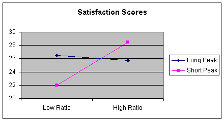
This is interesting data and
shows interaction. Customer satisfaction depends upon the what
combination of ratio and peak the customer was considering. In multiple
regression, when interaction is present, we say the relationship between
customer satisfaction and low or high ratio depends on length of the
peak.
Statistically, to validate the presence of interaction, we examine the ANOVA
table in Worksheet 4.5.2. There are three rows of interest. The Sample
row pertains to variation attributed to the peak factor; the Column row
pertains to variation attributed to the ratio factor; the Interaction row
pertains to variation attributed to the interaction of combinations of both
peak and ratio factors; and the Within row pertains to within group
variation (variation unexplained by peak period or ratio discount).
The first thing we test for is interaction in the Two-Factor ANOVA model. The
hypotheses are:
H0:
There is no interaction (Interaction is not important)
Ha: There is interaction (relationship between satisfaction and
length of peak period depends on ratio discount; which is the same as stating
the relationship between satisfaction and ratio discount depends on length of
peak period).
Since the p-value for Interaction (0.002749) is less than an alpha value of
0.01 (I am using the lower value of alpha to recognize that we are doing
multiple tests with the same data), we reject the null hypothesis and conclude
there is interaction in the data. Thus, the company needs to consider both the
length of the peak period as well as the discount ratio when setting peak/off
peak price discounts.
A
Situation without Interaction
A production firm
that assembles surgical kits for hospital operating rooms noticed that female
employees seem to assemble kits faster than male employees (this factor would
be the gender factor). If there is a significant gender effect, the company
would need to somehow recognize and respond to the different average assembly
times. There is another factor that must be considered: there are two methods
of assembly.
In this situation, the ANOVA model is used to determine if we can analyze
average assembly time with respect to each factor independent of the other, or
if we have to address interaction. If there is no interaction, the the average
assembly time for males can be compared to the average assembly time for
females . Likewise, if there is no interaction, then the average assembly time
for Method 1 can be compared to the average assembly time for Method 2. If
there is interaction, then averages involving combinations of the two factors
must be studied: average assembly time for males using Method 1; for males
using Method 2; for females using Method 1, and for females using Method 2. Worksheet 4.5.4 provides the data for
running the Two-Factor ANOVA model in Excel.
Worksheet 4.5.4
|
Method 1 |
Method 2 |
|
|
Male |
125 |
121 |
|
Male |
117 |
119 |
|
Male |
123 |
120 |
|
Female |
106 |
102 |
|
Female |
107 |
102 |
|
Female |
100 |
103 |
The Two-Factor ANOVA
is run in Excel as before. Select Tools, Data Analysis, ANOVA: Two-Factor
with Replication, and respond to the dialog box. . (In Excel 2007 select Data, then Data Analysis. From the pulldown menu select ANOVA: Two-Factor with Replication).
This time, there are three rows for the Sample or row factor, Gender. Worksheet
4.5.5 provides the result.
Worksheet 4.5.5
|
Anova: Two-Factor With Replication |
||||||
|
SUMMARY |
Method 1 |
Method 2 |
Total |
|||
|
Male |
||||||
|
Count |
3 |
3 |
6 |
|||
|
Sum |
365 |
360 |
725 |
|||
|
Average |
121.6667 |
120 |
120.8333 |
|||
|
Variance |
17.33333 |
1 |
8.166667 |
|||
|
Female |
||||||
|
Count |
3 |
3 |
6 |
|||
|
Sum |
313 |
307 |
620 |
|||
|
Average |
104.3333 |
102.3333333 |
103.3333 |
|||
|
Variance |
14.33333 |
0.333333333 |
7.066667 |
|||
|
Total |
||||||
|
Count |
6 |
6 |
||||
|
Sum |
678 |
667 |
||||
|
Average |
113 |
111.1666667 |
||||
|
Variance |
102.8 |
94.16666667 |
||||
|
ANOVA |
||||||
|
Source of Variation |
SS |
df |
MS |
F |
P-value |
F crit |
|
Sample |
918.75 |
1 |
918.75 |
111.3636 |
5.67E-06 |
5.317645 |
|
Columns |
10.08333 |
1 |
10.08333 |
1.222222 |
0.301061 |
5.317645 |
|
Interaction |
0.083333 |
1 |
0.083333 |
0.010101 |
0.922417 |
5.317645 |
|
Within |
66 |
8 |
8.25 |
|||
|
Total |
994.9167 |
11 |
||||
Also as before, with
Two-Factor Anova, we first test interaction. The hypotheses are:
H0:
There is no interaction (Interaction is not important)
Ha: There is interaction (relationship between assembly time and
gender depends on assembly method; which is the same as stating the
relationship between assembly time and assembly method depends on gender).
Since the p-value (0.922417)
is greater than 0.01, we do not reject the null hypothesis and conclude there
is no interaction.
Now we can independently test the factors. First, let's look at gender.
H0:
MeanMale = MeanFemale
Ha: MeanMale =/= MeanFemale
Since the p-value for the
Sample Factor (the row or gender factor) (5.67E-06) is less than 0.01, reject
the null hypothesis and conclude that the means are not equal. In this case, we
can use the top part of the ANOVA result to see which mean is less. The Male
mean is given in the total column for the Male data as 120.83 minutes per
surgical kit, and for the Female data, the mean is 103.3. The females are
significantly faster, on average, than the males.
Finally, we can test the assembly method factor. The hypotheses statements are:
H0: MeanMethod 1 = MeanMethod 2
Ha: MeanMethod 1 =/= MeanMethod 2
Since the p-value (0.301061)
for the Method factor (the Column factor), is greater than 0.01, do not reject
the null hypothesis. These is no significant difference in the average assembly
time for Method 1 compared to Method 2.
The company can now study the gender factor without regard to method of
assembly. Here is a picture of this situation:
Worksheet 4.5.6
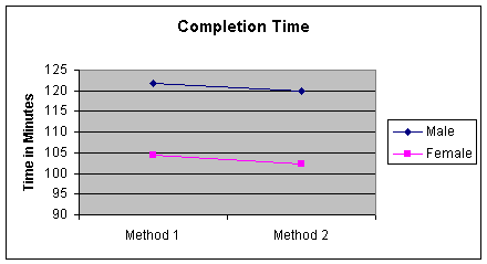
Note that the male averages are greater than the female averages, no matter
what the method of assembly - that is a picture of no interaction.
Two-Factor
Anova: Without Replication
You may have noticed
that you have two choices in the Data Analysis selections for Two-Factor ANOVA.
One is with replication (multiple rows for the factors being analyzed as we saw
in both of the previous examples), and one without replication. The
"without replication" can be used for problems such as the following.
A company employs three estimators in preparing bids for four different types
of construction jobs. The company is interested in determining if the
estimators are consistent in their bids. An experiment is created to have each
estimator independently prepare an estimate for Job 1, Job 2, Job 3 and Job 4.
So Estimator 1 prepares an estimate for Job 1, Estimator 2 prepares an estimate
for Job 1, and Estimator 3 prepares an estimate for Job 1; this is repeated for
Job 2, then Job 3, then Job 4.
The results are shown in Worksheet 4.5.7. Estimates are in millions of dollars.
Worksheet 4.5.7
|
Estimator 1 |
Estimator 2 |
Estimator 3 |
|
|
Job 1 |
4.6 |
4.9 |
4.1 |
|
Job 2 |
6.2 |
6.3 |
5.6 |
|
Job 3 |
5 |
5.4 |
5.1 |
|
Job 4 |
6.6 |
6.8 |
6.0 |
To analyze this problem with Two-Factor ANOVA, we select Tools, Data
Analysis, Anova: Two-Factor without Replication. (In Excel 2007 select
Data, then Data Analysis. From the
pulldown menu select ANOVA: Two-Factor
without Replication). Fill-in the entries on the dialog box,
and obtain the following output:
Worksheet 4.5.8
|
Anova: Two-Factor Without Replication |
||||||
|
SUMMARY |
Count |
Sum |
Average |
Variance |
||
|
Job 1 |
3 |
13.6 |
4.533333333 |
0.163333333 |
||
|
Job 2 |
3 |
18.1 |
6.033333333 |
0.143333333 |
||
|
Job 3 |
3 |
15.5 |
5.166666667 |
0.043333333 |
||
|
Job 4 |
3 |
19.4 |
6.466666667 |
0.173333333 |
||
|
Estim'r 1 |
4 |
22.4 |
5.6 |
0.906666667 |
||
|
Estim'r 2 |
4 |
23.4 |
5.85 |
0.736666667 |
||
|
Estim'r 3 |
4 |
20.8 |
5.2 |
0.673333333 |
||
|
ANOVA |
||||||
|
Source of Variation |
SS |
df |
MS |
F |
P-value |
F crit |
|
Rows |
6.763333333 |
3 |
2.254444444 |
72.46428571 |
4.1954E-05 |
4.757055194 |
|
Columns |
0.86 |
2 |
0.43 |
13.82142857 |
0.005672508 |
5.143249382 |
|
Error |
0.186666667 |
6 |
0.031111111 |
|||
|
Total |
7.81 |
11 |
The hypothesis test of
interest is as follows:
H0:
MeanEstimator 1 = MeanEstimator 2 = MeanEstimator 3
Ha: At least two means are not equal
The
factor of interest is Estimator, the column factor. Since the p-value
(0.005672508) is less than alpha of 0.05 (only one test is being done with the
data), we do reject the null hypothesis and conclude that there is a
significant difference in the mean estimates. This finding would have to be
addressed by management .
This model takes into consideration the fact that the jobs themselves had
variability - Type 1 Jobs are smaller than Type 4 Jobs, for example. The
Two-Factor ANOVA model without replication accounts for the variability of the
row factor so that the column factor can be more effectively studied.
If we would have assumed that there is no difference in the job types, then we
would assumed that jobs were independently and randomly assigned to each
estimator. This is the One-Factor ANOVA we studied in Module Notes 4.4.
Worksheet 4.5.9 shows the results of the One-Factor ANOVA.
Worksheet 4.5.9
|
Anova: Single Factor |
||||||
|
SUMMARY |
||||||
|
Groups |
Count |
Sum |
Average |
Variance |
||
|
Estim'r 1 |
4 |
22.4 |
5.6 |
0.906666667 |
||
|
Estim'r 2 |
4 |
23.4 |
5.85 |
0.736666667 |
||
|
Estim'r 3 |
4 |
20.8 |
5.2 |
0.673333333 |
||
|
ANOVA |
||||||
|
Source of Variation |
SS |
df |
MS |
F |
P-value |
F crit |
|
Between Groups |
0.86 |
2 |
0.43 |
0.556834532 |
0.591564315 |
4.256492048 |
|
Within Groups |
6.95 |
9 |
0.772222222 |
|||
|
Total |
7.81 |
11 |
Note carefully that the
p-value for Between Group variation (the Estimator factor) is now greater than
0.05, so we would not reject the null hypothesis and conclude the average
estimates are the same. In this case, the wrong model would lead us to an
erroneous conclusion.
Summary
The two factor ANOVA
models are very powerful additions to the Single Factor ANOVA. The assumptions
with the two-factor models are that populations from which the samples were
drawn are normal and the variances are equal. The normality assumption is not
critical in the presence of large sample sizes, and the variance assumption is
not critical when there are equal sample sizes for the factor level
combinations. However, when we work with small samples, samples with unequal
sizes in the factor level combinations, and/or when the sample indicates
extreme values (skewed data), we should revert to nonparametric techniques, as
will be described in Module Notes 4.6.
The two-factor ANOVA with replication assumes that observations are randomly
and independently assigned to each group of the two factors. The two-factor
ANOVA does not make that assumption and is used when one wants to control for
the variability of the row factor.
Readings:
Ken
Black. Business Statistics for Contemporary Decision Making. Fourth Edition,
Wiley. Chapter 10 & 11
D. Groebner, P. Shannon, P.
Fry & K. Smith. Business Statistics:
A Decision Making Approach, Fifth Edition, Prentice Hall, Chapter 10
Levine,
D., Berenson, M. & Stephan, D. (1999). Statistics for Managers Using
Microsoft Excel (2nd. ed.). Upper Saddle River, NJ: Prentice-Hall, Chapter
10.
Mason, R., Lind, D. &
Marchal, W. (1999). Statistical Techniques in Business and Economics (10th.
ed.). Boston: Irwin McGraw Hill, Chapter
11.