Understanding the Graphical representation of Motion.

The Goal

The purpose of this lab is to elucidate the relationship between the motion of an object and a graphical representation of this motion (a graph of position versus time for the moving object).

Prerequisites

“Physics for Scientists and Engineers” R.D. Knight: Chapters 1, 2.1-2.5

Equipment

- PC

- Science Workshop Interface

- Motion sensor with base and support rod

Brief Theoretical Overview

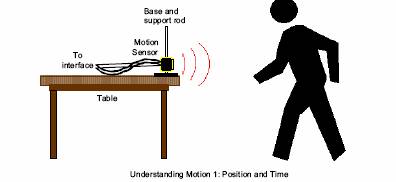
To describe the motion of any object you have to define a suitable reference point and introduce an appropriate coordinate system. In this particular lab you will have deal with one-dimensional motion, and thus you need to use the only coordinate axis. The full description of the motion then would be provided by knowing an exact position of the object at any arbitrary moment of time. The motion sensor uses pulses of ultrasound that reflect from the moving object to determine its current position. The current position of the moving object is measured many times every second. The results of measurements are plotted in the PC screen as a function of elapsed time.

The graph of position versus time gives us a graphical representation of the motion. Using this graph you can determine how other characteristics of motion (velocity and acceleration) change. Reminder: the rate at which a position changes is just a velocity of the object in motion. By analogy, the rate at which a velocity changes, is an acceleration of the object.

Procedure

You will be the object in motion in this lab. You will move with different speeds over straight line back and forth with respect to the motion sensor. The motion sensor will measure your position as a function of time. The Science Workshop Interface (computer program) will plot the graph of your position versus time on the PC screen. The real challenge in this activity is to move in such a way that a plot of your motion on the screen matches the prepared line that is already there.

You do not need neither to set up any equipment nor to calibrate motion sensor in this lab – everything is already prepared for you. You have to position the computer monitor in such a way that you can see the screen moving away from the motion sensor. Note: you will be moving backwards for a meter or two from the monitor – clear the area behind you for at least two meters (it is about 6 feet).

Now you are ready to work.

1. From the prepared graph on the PC screen determine your initial position X₀.

2. Make a few trials to verify that you correctly determined the initial position. To do that you have to start recording being at rest at the initial position. To start recording click on the REC button. Data recording will begin almost immediately. You will hear a faint clicking noise from the motion sensor. To stop recording click STOP button. Note: the graph can show up to three different runs simultaneously. To delete a run of data, click on the run in the Data list in the Experiment Setup window and press the “delete” key on the keyboard. Note: this exercise is easier to do if you have a partner to run the computer while you move.

3. From the prepared graph on the PC screen find out how far you should move and how long your motion should last.

4. Try to reproduce the prepared line in the screen.

5. Repeat your trip a few times to obtain as close match as possible.

Analysis of data

1. Draw you best matched graph position versus time in your Lab Report.

2. Determine how your velocity changed during your trip. Draw corresponding graph velocity versus time under graph position versus time. Note: the time axes have to have the same scale.

3. Find out numerical value of velocity at different stages of your motion. You can do this in two different ways:

- manually, determining the slop of your position versus time graph;

- using statistical tools in the graph. Click “Statistics” button and then click “Autoscale” button to resize the graph to fit the data. Use the mouse to click-and-draw a rectangle around an appropriate section of your plot. Use the Statistics menu button in the Statistics area of the graph. Select “Linear Fit” from the Curve Fit menu to display the slope of the selected region of your position versus time plot. The a2 coefficient of the equation in the Status area is the slope of the selected region of motion.

4. Determine how your acceleration was changing during your trip. Qualitatively draw corresponding graph acceleration versus time under graph velocity versus time. Note: the time axes have to have the same scale.

5. Estimate how well your plot of motion fits the prepared plot on the screen. Note, that you do not have to use any sophisticated statistical calculations for that – just try to give qualitative estimation. What are the possible explanations of differences between these two plots? Write a short essay (3-5 statements) about that.

6. Estimate the accuracy of numerical values for the velocities and accelerations, obtained by you, at the different stages of your trip.

Lab Report Preparation

Write an appropriate lab report. It has to contain

1. Your name and name of all your partners, date and time of work.

2. Name of the lab (title).

3. Goal of the lab.

4. List of equipment used in the lab.

5. Obtained data with detailed analysis.